Authors: Mehmed Kantardzic
Data Mining (10 page)
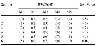
and if the window for analysis of the time-series is five, then it is possible to reorganize the input data into a tabular form with six samples, which is more convenient (standardized) for the application of data-mining techniques. Transformed data are given in Table
2.1
.
TABLE 2.1.
Transformation of Time Series to Standard Tabular Form (Window = 5)
The best time lag must be determined by the usual evaluation techniques for a varying complexity measure using independent test data. Instead of preparing the data once and turning them over to the data-mining programs for prediction, additional iterations of data preparation have to be performed. Although the typical goal is to predict the next value in time, in some applications, the goal can be modified to predict values in the future, several time units in advance. More formally, given the time-dependent values t(n − i), … , t(n), it is necessary to predict the value t(n + j). In the previous example, taking j = 3, the new samples are given in Table
2.2
.
TABLE 2.2.
Time-Series Samples in Standard Tabular Form (Window = 5) with Postponed Predictions (j = 3)

In general, the further in the future, the more difficult and less reliable is the forecast. The goal for a time series can easily be changed from predicting the next value in the time series to classification into one of predefined categories. From a data-preparation perspective, there are no significant changes. For example, instead of predicted output value t(i + 1), the new classified output will be binary:
T
for t(i + 1) ≥ threshold value and
F
for t(i + 1) < threshold value.
The time units can be relatively small, enlarging the number of artificial features in a tabular representation of time series for the same time period. The resulting problem of high dimensionality is the price paid for precision in the standard representation of the time-series data.
In practice, many older values of a feature may be historical relics that are no longer relevant and should not be used for analysis. Therefore, for many business and social applications, new trends can make old data less reliable and less useful. This leads to a greater emphasis on recent data, possibly discarding the oldest portions of the time series. Now we are talking not only of a fixed window for the presentation of a time series but also on a fixed size for the data set. Only the n most recent cases are used for analysis, and, even then, they may not be given equal weight. These decisions must be given careful attention and are somewhat dependent on knowledge of the application and past experience. For example, using 20-year-old data about cancer patients will not give the correct picture about the chances of survival today.
Besides standard tabular representation of time series, sometimes it is necessary to additionally preprocess raw data and summarize their characteristics before application of data-mining techniques. Many times it is better to predict the difference t(n + 1) − t(n) instead of the absolute value t(n + 1) as the output. Also, using a ratio, t(n + 1)/t(n), which indicates the percentage of changes, can sometimes give better prediction results. These transformations of the predicted values of the output are particularly useful for logic-based data-mining methods such as decision trees or rules. When differences or ratios are used to specify the goal, features measuring differences or ratios for input features may also be advantageous.
Time-dependent cases are specified in terms of a goal and a time lag or a window of size m. One way of summarizing features in the data set is to average them, producing MA. A single average summarizes the most recent m feature values for each case, and for each increment in time, its value is

Knowledge of the application can aid in specifying reasonable sizes for m. Error estimation should validate these choices. MA weight all time points equally in the average. Typical examples are MA in the stock market, such as 200 days MA for the DOW or NASDAQ. The objective is to smooth neighboring time points by an MA to reduce the random variation and noise components

Another type of average is an
exponential moving average
(EMA) that gives more weight to the most recent time periods. It is described recursively as


where p is a value between 0 and 1. For example, if p = 0.5, the most recent value t(i) is equally weighted with the computation for all previous values in the window, where the computation begins with averaging the first two values in the series. The computation starts with the following two equations:


As usual, application knowledge or empirical validation determines the value of p. The exponential MA has performed very well for many business-related applications, usually producing results superior to the MA.
An MA summarizes the recent past, but spotting a change in the trend of the data may additionally improve forecasting performances. Characteristics of a trend can be measured by composing features that compare recent measurements with those of the more distant past. Three simple comparative features are
1.
t(i) − MA(i, m), the difference between the current value and an MA,
2.
MA(i, m) − MA(i − k, m), the difference between two MAs, usually of the same window size, and
3.
t(i)/MA(i, m), the ratio between the current value and an MA, which may be preferable for some applications.
In general, the main components of the summarizing features for a time series are
1.
current values,
2.
smoothed values using MA, and
3.
derived trends, differences, and ratios.
The immediate extension of a univariate time series is to a multivariate one. Instead of having a single measured value at time i, t(i), multiple measurements t[a(i), b(j)] are taken at the same time. There are no extra steps in data preparation for the multivariate time series. Each series can be transformed into features, and the values of the features at each distinct time A(i) are merged into a sample i. The resultant transformations yield a standard tabular form of data such as the table given in Figure
2.5
.
Figure 2.5.
Tabulation of time-dependent features. (a) Initial time-dependent data; (b) samples prepared for data mining with time window = 3.
