Read In Pursuit of the Unknown Online
Authors: Ian Stewart
In Pursuit of the Unknown (55 page)
Â
Â
It models how a population of living creatures changes from one generation to the next, when there are limits to the available resources.
It is one of the simplest equations that can generate deterministic chaos â apparently random behaviour with no random cause.
The realisation that simple nonlinear equations can create very complex dynamics, and that apparent randomness may conceal hidden order. Popularly known as chaos theory, this discovery has innumerable applications throughout the sciences including the motion of the planets in the Solar System, weather forecasting, population dynamics in ecology, variable stars, earthquake modelling, and efficient trajectories for space probes.
T
he metaphor of the balance of nature trips readily off the tongue as a description of what the world would do if nasty humans didn't keep interfering. Nature, left to its own devices, would settle down to a state of perfect harmony. Coral reefs would always harbour the same species of colourful fish in similar numbers, rabbits and foxes would learn to share the fields and woodlands so that the foxes would be well fed, most rabbits would survive, and neither population would explode or crash. The world would settle down to a fixed state and stay there. Until the next big meteorite, or a supervolcano, upset the balance.
It's a common metaphor, perilously close to being a cliché. It's also highly misleading. Nature's balance is distinctly wobbly.
We've been here before. When Poincaré was working on King Oscar's prize, the conventional wisdom held that a stable Solar System is one in which the planets follow much the same orbits forever, give or take a harmless bit of jiggling. Technically this is not a steady state, but one in which each planet repeats similar motions over and over again, subject to minor disturbances caused by all the others, but not deviating hugely from what it would have done without them. The dynamics is âquasiperiodic' â combining several separate periodic motions whose periods are not all multiples of the same time interval. In the realm of planets, that's as close to âsteady' as anyone can hope for.
But the dynamics wasn't like that, as Poincaré belatedly, and to his cost, found out. It could, in the right circumstances, be chaotic. The equations had no explicit random terms, so that in principle the present state completely determined the future state, yet paradoxically the actual motion could appear to be random. In fact, if you asked coarse-grained questions like âwhich side of the Sun will it be on?', the answer could be a genuinely random series of observations. Only if you could look infinitely closely would you be able to see that the motion really was completely determined.
This was the first intimation of what we now call âchaos', which is short for âdeterministic chaos', and quite different from ârandom' â even though that's what it can look like. Chaotic dynamics has hidden patterns, but
they're subtle; they differ from what we might naturally think of measuring. Only by understanding the causes of chaos can we extract those patterns from an irregular mishmash of data.
As always in science, there were a few isolated precursors, generally viewed as minor curiosities unworthy of serious attention. Only in the 1960s did mathematicians, physicists, and engineers begin to realise just how natural chaos is in dynamics, and how radically it differs from anything envisaged in classical science. We are still learning to appreciate what that tells us, and what to do about it. But already chaotic dynamics, âchaos theory' in popular parlance, pervades most areas of science. It may even have things to tell us about economics and the social sciences. It's not the answer to everything: only critics ever claimed it was, and that was to make it easier to shoot it down. Chaos has survived all such attacks, and for a good reason: it is absolutely fundamental to all behaviour governed by differential equations, and those are the basic stuff of physical law.
There is chaos in biology, too. One of the first to appreciate that this might be the case was the Australian ecologist Robert May, now Lord May of Oxford and a former president of the Royal Society. He sought to understand how the populations of various species change over time in natural systems such as coral reefs and woodlands. In 1975 May wrote a short article for the journal
Nature
, pointing out that the equations typically used to model changes to animal and plant populations could produce chaos. May didn't claim that the models he was discussing were accurate representations of what real populations did. His point was more general: chaos was natural in models of that kind, and this had to be borne in mind.
The most important consequence of chaos is that irregular behaviour need not have irregular causes. Previously, if ecologists noticed that some population of animals was fluctuating wildly, they would look for some external cause â also presumed to be fluctuating wildly, and generally labelled ârandom'. The weather, perhaps, or a sudden influx of predators from elsewhere. May's examples showed that the internal workings of the animal populations could generate irregularity without outside help.
His main example was the equation that decorates the opening of this chapter. It is called the logistic equation, and it is a simple model of a population of animals in which the size of each generation is determined by the previous one. âDiscrete' means that the flow of time is counted in generations, and is thus an integer. So the model is similar to a differential
equation, in which time is a continuous variable, but conceptually and computationally simpler. The population is measured as a fraction of some overall large value, and can therefore be represented by a real number that lies between 0 (extinction) and 1 (the theoretical maximum that the system can sustain). Letting time
t
tick in integer steps, corresponding to generations, this number is
x
t
in generation
t
. The logistic equation states that
x
t + 1
=
Kx
t
(1 â
x
t
)
where
k
is a constant. We can interpret
k
as the growth rate of the population when diminishing resources do not slow it down.
1
We start the model at time 0 with an initial population
x
0
. Then we use the equation with
t
= 0 to calculate
x
1
, then we set
t
= 1 and compute
x
2
, and so on. Without even doing the sums we can see straight away that, for any fixed growth rate
k
, the population size of generation zero completely determines the sizes of all succeeding generations. So the model is
deterministic
: knowledge of the present determines the future uniquely and exactly.
So what
is
the future? The âbalance of nature' metaphor suggests that the population should settle to a steady state. We can even calculate what that steady state should be: just set the population at time
t
+ 1 to be the same as that at time
t
. This leads to two steady states: populations 0 and 1-1/
k
. A population of size 0 is extinct, so the other value should apply to an existing population. Unfortunately, although this is a steady state, it can be unstable. If it is, then in practice you'll never see it: it's like trying to balance a pencil vertically on its sharpened point. The slightest disturbance will cause it to topple. The calculations show that the steady state is unstable when
k
is bigger than 3.
What, then,
do
we see in practice?
Figure 58
shows a typical âtime series' for the population when
k
= 4. It's not steady: it's all over the place. However, if you look closely there are hints that the dynamics is not completely random. Whenever the population gets really big, it immediately crashes to a very low value, and then grows in a regular manner (roughly exponentially) for the next two or three generations: see the short arrows in
Figure 58
. And something interesting happens whenever the population gets close to 0.75 or thereabouts: it oscillates alternately above and below that value, and the oscillations grow giving a characteristic zigzag shape, getting wider towards the right: see the longer arrows in the figure.
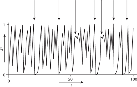
Fig 58
Chaotic oscillations in a model animal population. Short arrows show crashes followed by short-term exponential growth. Longer arrows show unstable oscillations.
Despite these patterns, there is a sense in which the behaviour is truly random â but only when you throw away some of the detail. Suppose we assign the symbol H (heads) whenever the population is bigger than 0.5, and T (tails) when it's less than 0.5. This particular set of data begins with the sequence THTHTHHTHHTTHH and continues unpredictably, just like a random sequence of coin tosses. This way of coarsening the data, by looking at specific ranges of values and noting only which range the population belongs to, is called symbolic dynamics. In this case, it is possible to prove that, for almost all initial population values
x
0
, the sequence of heads and tails is in all respects like a typical sequence of random tosses of a fair coin. Only when we look at the exact values do we start to see some patterns.
It's a remarkable discovery. A dynamical system can be completely deterministic, with visible patterns in detailed data, yet a coarse-grained view of the same data can be random â in a provable, rigorous sense. Determinism and randomness are not opposites. In some circumstances, they can be entirely compatible.
May didn't invent the logistic equation, and he didn't discover its astonishing properties. He didn't claim to have done either of those things. His aim was to alert workers in the life sciences, especially ecologists, to the remarkable discoveries emerging in the physical sciences and mathematics: discoveries that fundamentally change the way scientists should think about observational data. We humans may have
trouble solving equations based on simple rules, but nature doesn't have to solve the equations the way we do. It just obeys the rules. So it can do things that strike us as being complicated, for simple reasons.
Chaos emerged from a topological approach to dynamics, orchestrated in particular by the American mathematician Stephen Smale and the Russian mathematician Vladimir Arnold in the 1960s. Both were trying to find out what types of behaviour were typical in differential equations. Smale was motivated by Poincaré's strange results on the three-body problem (
Chapter 4
), and Arnold was inspired by related discoveries of his former research supervisor Andrei Kolmogorov. Both quickly realised why chaos is common: it is a natural consequence of the geometry of differential equations, as we'll see in a moment.
As interest in chaos spread, examples were spotted lurking unnoticed in earlier scientific papers. Previously considered to be just isolated weird effects, these examples now slotted into a broader theory. In the 1940s the English mathematicians John Littlewood and Mary Cartwright had seen traces of chaos in electronic oscillators. In 1958 Tsuneji Rikitake of Tokyo's Association for the Development of Earthquake Prediction had found chaotic behaviour in a dynamo model of the Earth's magnetic field. And in 1963 the American meteorologist Edward Lorenz had pinned down the nature of chaotic dynamics in considerable detail, in a simple model of atmospheric convection motivated by weather-forecasting. These and other pioneers had pointed the way; now all of their disparate discoveries were starting to fit together.
In particular, the circumstances that led to chaos, rather than something simpler, turned out to be geometric rather than algebraic. In the logistic model with
k
= 4, both extremes of the population, 0 and 1, move to 0 in the next generation, while the midpoint, , moves to 1. So at each time-step the interval from 0 to 1 is stretched to twice its length, folded in half, and slapped down in its original location. This is what a cook does to dough when making bread, and by thinking about dough being kneaded, we gain a handle on chaos. Imagine a tiny speck in the logistic dough â a raisin, say. Suppose that it happens to lie on a periodic cycle, so that after a certain number of stretch-and-fold operations it returns to where it started. Now we can see why this point is unstable. Imagine another raisin, initially very close to the first one. Each stretch moves it further away. For a time, though, it doesn't move far enough away to stop tracking the first raisin. When the dough is folded, both raisins end up in the same layer. So next time, the second raisin has moved even further away from the first. This is why the periodic state is unstable:
stretching moves all nearby points
away
from it, not towards it. Eventually the expansion becomes so great that the two raisins end up in different layers when the dough is folded. After that, their fates are pretty much independent of each other. Why does a cook knead dough? To mix up the ingredients (including trapped air). If you mix stuff up, the individual particles have to move in a very irregular way. Particles that start close together end up far apart; points far apart may be folded back to be close together. In short, chaos is the natural result of
mixing
.