Data Mining (81 page)
Authors: Mehmed Kantardzic
Theory and practical applications both show that all approaches in the validation of clustering results have a subjective component. Hence, little in the way of “gold standards” exists in clustering evaluation. Recent studies in cluster analysis suggest that a user of a clustering algorithm should always keep the following issues in mind:
1.
Every clustering algorithm will find clusters in a given data set whether they exist or not; the data should, therefore, be subjected to tests for clustering tendency before applying a clustering algorithm, followed by a validation of the clusters generated by the algorithm.
2.
There is no best clustering algorithm; therefore, a user is advised to try several algorithms on a given data set.
It is important to remember that cluster analysis is an exploratory tool; the outputs of clustering algorithms only suggest or sometimes confirm hypotheses, but never prove any hypothesis about natural organization of data.
9.9 REVIEW QUESTIONS AND PROBLEMS
1.
Why is the validation of a clustering process highly subjective?
2.
What increases the complexity of clustering algorithms?
3.
(a)
Using MND distance, distribute the input samples given as 2-D points A(2, 2), B(4, 4), and C(7, 7) into two clusters.
(b)
What will be the distribution of samples in the clusters if samples D(1, 1), E(2, 0), and F(0, 0) are added?
4.
Given 5-D numeric samples A = (1, 0, 2, 5, 3) and B = (2, 1, 0, 3, −1), find
(a)
the Eucledian distance between points;
(b)
the city-block distance;
(c)
the Minkowski distance for p = 3; and
(d)
the cosine-correlation distance.
5.
Given 6-D categorical samples C = (A, B, A, B, A, A) and D = (B, B, A, B, B, A), find
(a)
an SMC of the similarity between samples;
(b)
Jaccard’s coefficient; and
(c)
Rao’s coefficient
6.
Given a set of 5-D categorical samples
A = (1, 0, 1, 1, 0)
B = (1, 1, 0, 1, 0)
C = (0, 0, 1, 1, 0)
D = (0, 1, 0, 1, 0)
E = (1, 0, 1, 0, 1)
F = (0, 1, 1, 0, 0)
(a)
Apply agglomerative hierarchical clustering using
(i)
single-link similarity measure based on Rao’s coefficient; and
(ii)
complete-link similarity measure based on SMC.
(b)
Plot the dendrograms for the solutions to parts (i) and (ii) of (a).
7.
Given the samples X1 = {1, 0}, X2 = {0, 1}, X3 = {2, 1}, and X4 = {3, 3}, suppose that the samples are randomly clustered into two clusters C1 = {X1, X3} and C2 = {X2, X4}.
(a)
Apply one iteration of the K-means partitional-clustering algorithm, and find a new distribution of samples in clusters. What are the new centroids? How can you prove that the new distribution of samples is better than the initial one?
(b)
What is the change in the total square-error?
(c)
Apply the second iteration of the K-means algorithm and discuss the changes in clusters.
8.
For the samples in Problem 7, apply iterative clustering with the threshold value for cluster radius T = 2. What is the number of clusters and samples distribution after the first iteration?
9.
Suppose that the samples in Problem 6 are distributed into two clusters:
C1 = {A, B, E} and C2 = {C, D, F}.
Using K-nearest neighbor algorithm, find the classification for the following samples:
(a)
Y = {1 ,1 ,0 ,1 ,1} using K = 1
(b)
Y = {1 ,1 ,0 ,1 ,1} using K = 3
(c)
Z = {0, 1, 0, 0, 0} using K = 1
(d)
Z = {0, 1, 0, 0, 0} using K = 5.
10.
Implement the hierarchical agglomerative algorithm for samples with categorical values using the SMC measure of similarity.
11.
Implement the partitional K-means clustering algorithm. Input samples are given in the form of a flat file.
12.
Implement the incremental-clustering algorithm with iterations. Input samples are given in the form of a flat file.
13.
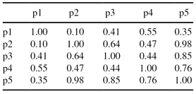
Given the similarity matrix between five samples:
(a)
Use the similarity matrix in the table to perform
complete link
hierarchical clustering. Show your results by drawing a dendrogram. The dendrogram should clearly show the order in which the points are merged.
(b)
How many clusters exist if the threshold similarity value is 0.5. Give the elements of each cluster.
(c)
If DBSCAN algorithm is applied with threshold similarity of 0.6, and MinPts ≥ 2 (required density), what are
core
,
border
,and
noise
points in the set of points
p
i
given in the table. Explain.

14.
Given the points x1 = {1, 0}, x2 = {0,1}, x3 = {2, 1}, and x4 = {3, 3}, suppose that these points are randomly clustered into two clusters: C1 = {x1, x3} and C2 = {x2, x4}. Apply one iteration of
K-means partitional clustering algorithm
and find new distribution of elements in clusters. What is the change in
total square-error
?
15.
Answer True/False to the following statements. Discuss your answer if necessary.
(a)
Running K-means with different initial seeds is likely to produce different results.
(b)
Initial cluster centers have to be data points.
(c)
Clustering stops when cluster centers are moved to the mean of clusters.
(d)
K-means can be less sensitive to outliers if standard deviation is used instead of the average.
(e)
K-means can be less sensitive to outliers if median is used instead of the average.
16.
Identify the clusters in the Figure below using the center-, contiguity-, and density-based clustering. Assume center-based means
K-means,
contiguity-based means single link hierarchical and density-based means
DBSCAN
. Also indicate the number of clusters for each case, and give a brief indication of your reasoning. Note that darkness or the number of dots indicates density.

17.
Derive the mathematical relationship between cosine similarity and Euclidean distance when each data object has an L2 (Euclidean) length of 1.
18.
Given a similarity measure with values in the interval [0, 1], describe two ways to transform this similarity value into a
dissimilarity
value in the interval [0, ∞].
19.
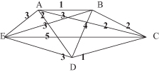
Distances between samples (A, B, C, D, and E) are given in a graphical form:
Determine single-link and complete-link dendograms for the set of the samples.

20.
There is a set S consisting of six points in the plane shown as below, a = (0, 0), b = (8, 0), c = (16, 0), d = (0, 6), e = (8, 6), f = (16, 6). Now we run the k-means algorithm on those points with k = 3. The algorithm uses the Euclidean distance metric (i.e., the straight line distance between two points) to assign each point to its nearest centroid. Also we define the following:
- 3-starting configuration
is a subset of three starting points from S that form the initial centroids, for example, {a, b, c}. - 3-partition
is a partition of S into k nonempty subsets, for example, {a, b, e}, {c, d}, {f} is a 3-partition.(a)
How many 3-starting configurations are there?(b)
Fill in the last two columns of the following table.3-partition An example of a 3-starting configuration that can arrive at the 3-partition after 0 or more iterations of k-means Number of unique 3-starting configurations {a,b} {d,e} {c,f} {a} {d} {b, c, e, f} {a, b, d} {c} {e, f} {a, b} {d} {c, e, f}
9.10 REFERENCES FOR FURTHER STUDY
Filippone, M., F. Camastra, F. Masulli, S. Rovetta, A Survey of Kernel and Spectral Methods for Clustering,
Pattern Recognition
, Vol. 41, 2008, pp. 176–190.
Clustering algorithms are a useful tool to explore data structures and have been employed in many disciplines. The focus of this paper is the partitioning clustering problem with a special interest in two recent approaches: kernel and spectral methods. The aim of this paper is to present a survey of kernel and spectral clustering methods, two approaches that are able to produce nonlinear separating hypersurfaces between clusters. The presented kernel clustering methods are the kernel version of many classical clustering algorithms, for example,
K
-means, SOM, and neural gas. Spectral clustering arises from concepts in spectral graph theory and the clustering problem is configured as a graph-cut problem where an appropriate objective function has to be optimized.
Han, J., M. Kamber,
Data Mining: Concepts and Techniques
, 2nd edition, Morgan Kaufmann, San Francisco, CA, 2006.
This book gives a sound understanding of data-mining principles. The primary orientation of the book is for database practitioners and professionals with emphasis on OLAP and data warehousing. In-depth analysis of association rules and clustering algorithms is the additional strength of the book. All algorithms are presented in easily understood pseudo-code and they are suitable for use in real-world, large-scale data-mining projects including advanced applications such as Web mining and text mining.
Hand, D., H. Mannila, P. Smith,
Principles of Data Mining
, MIT Press, Cambridge, MA, 2001.
The book consists of three sections. The first, foundations, provides a tutorial overview of the principles underlying data-mining algorithms and their applications. The second section, data-mining algorithms, shows how algorithms are constructed to solve specific problems in a principled manner. The third section shows how all of the preceding analyses fit together when applied to real-world data-mining problems.
Jain, A. K., M. N. Murty, P. J. Flynn, Data Clustering: A Review,
ACM Computing Surveys
, Vol. 31, No. 3, September 1999, pp. 264–323.
Although there are several excellent books on clustering algorithms, this review paper will give the reader enough details about the state-of-the-art techniques in data clustering, with an emphasis on large data sets problems. The paper presents the taxonomy of clustering techniques and identifies crosscutting themes, recent advances, and some important applications. For readers interested in practical implementation of some clustering methods, the paper offers useful advice and a large spectrum of references.