Antifragile: Things That Gain from Disorder (83 page)
Read Antifragile: Things That Gain from Disorder Online
Authors: Nassim Nicholas Taleb
Let us apply this analysis to how planners make the mistakes they make, and why deficits tend to be worse than planned:
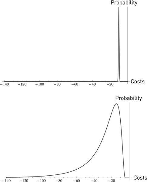
FIGURE 36
.
The gap between predictions and reality:
probability distribution of outcomes from costs of projects in the minds of planners (top) and in reality (bottom). In the first graph they assume that the costs will be both low and quite certain. The graph on the bottom shows outcomes to be both worse and more spread out, particularly with higher possibility of unfavorable outcomes. Note the fragility increase owing to the swelling left tail.
This misunderstanding of the effect of uncertainty applies to government deficits, plans that have IT components, travel time (to a lesser degree), and many more. We will use the same graph to show model error from underestimating fragility by assuming that a parameter is constant when it is random. This is what plagues bureaucrat-driven economics (next discussion).
WHERE MOST ECONOMIC MODELS FRAGILIZE AND BLOW PEOPLE UP

When I said “technical” in the main text, I may have been fibbing. Here I am not.
The Markowitz incoherence:
Assume that someone tells you that the probability of an event is exactly zero. You ask him where he got this from. “Baal told me” is the answer. In such case, the person is coherent, but would be deemed unrealistic by non-Baalists. But if on the other hand, the person tells you “I
estimated
it to be zero,” we have a problem. The person is both unrealistic and inconsistent. Something estimated needs to have an estimation error. So probability cannot be zero if it is estimated, its lower bound is linked to the estimation error; the higher the estimation error, the higher the probability, up to a point. As with Laplace’s argument of total ignorance, an infinite estimation error pushes the probability toward ½.
We will return to the implication of the mistake; take for now that anything estimating a parameter and then putting it into an equation is different from estimating the equation across parameters (same story as the health of the grandmother, the average temperature, here “estimated” is irrelevant, what we need is average health across temperatures). And Markowitz showed his incoherence by starting his “semi-nal” paper with “Assume you know
E
and
V
” (that is, the expectation and the variance). At the end of the paper he accepts that they need to be estimated, and what is worse, with a combination of statistical techniques and the “judgment of practical men.” Well, if these parameters need to be estimated, with an error, then the derivations need to be written differently and, of course, we would have no paper—and no Markowitz paper, no blowups, no modern finance, no fragilistas teaching junk to students.… Economic models are extremely fragile to assumptions, in the sense that a slight alteration in these assumptions can, as we will see, lead to extremely consequential differences in the results. And, to make matters worse, many of these models are “back-fit” to assumptions, in the sense that the hypotheses are selected to make the math work, which makes them ultrafragile and ultrafragilizing.
Simple example:
Government deficits.
We use the following deficit example owing to the way calculations by governments and government agencies currently miss convexity terms (and have a hard time accepting it). Really, they don’t take them into account. The example illustrates:
(a) missing the stochastic character of a variable known to affect the model but deemed deterministic (and fixed), and
(b)
F,
the function of such variable, is convex or concave with respect to the variable.
Say a government estimates unemployment for the next three years as averaging 9 percent; it uses its econometric models to issue a forecast balance
B
of a two-hundred-billion deficit in the local currency. But it misses (like almost everything in economics) that unemployment is a stochastic variable. Employment over a three-year period has fluctuated by 1 percent on average. We can calculate the effect of the error with the following:
Unemployment at 8%, Balance
B
(8%) = −75 bn (improvement of 125 bn)
Unemployment at 9%, Balance
B
(9%)= −200 bn
Unemployment at 10%, Balance
B
(10%)= −550 bn (worsening of 350 bn)
The concavity bias, or negative convexity bias, from underestimation of the deficit is −112.5 bn, since ½ {
B
(8%) +
B
(10%)} = −312 bn, not −200 bn. This is the exact case of the
inverse philosopher’s stone
.
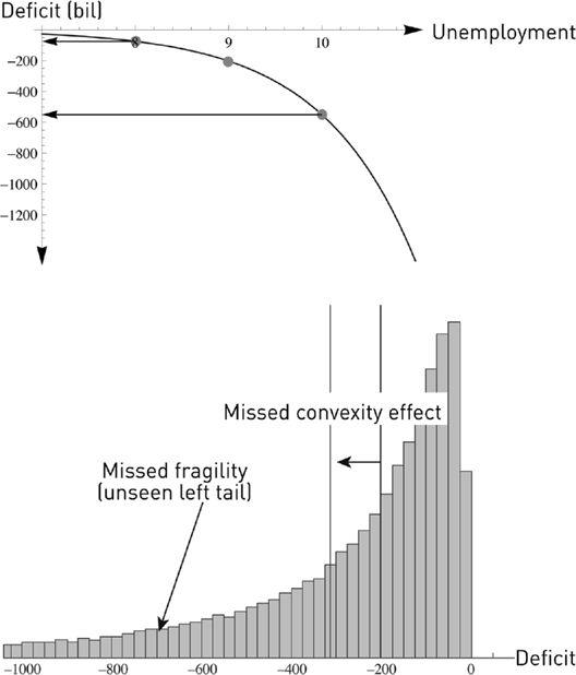
FIGURE 37.
Nonlinear transformations allow the detection of both model convexity bias and fragility.
Illustration of the example: histogram from Monte Carlo simulation of government deficit as a left-tailed random variable simply as a result of randomizing unemployment, of which it is a concave function. The method of point estimate would assume a Dirac stick at −200, thus underestimating both the
expected
deficit (−312) and the tail fragility of it. (From Taleb and Douady, 2012).
For almost two hundred years, we’ve been talking about an idea by the economist David Ricardo called “comparative advantage.” In short, it says that a country should have a certain policy based on its comparative advantage in wine or clothes. Say a country is good at both wine and clothes, better than its neighbors with whom it can trade freely. Then the visible
optimal
strategy would be to specialize in either wine or clothes, whichever fits the best and minimizes opportunity costs. Everyone would then be happy. The analogy by the economist Paul Samuelson is that if someone happens to be the best doctor in town and, at the same time, the best secretary,
then it would be preferable to be the higher-earning doctor—as it would minimize opportunity losses—and let someone else be the secretary and buy secretarial services from him.
I agree that there are benefits in
some
form of specialization, but not from the models used to prove it. The flaw with such reasoning is as follows. True, it would be inconceivable for a doctor to become a part-time secretary just because he is good at it. But, at the same time, we can safely assume that being a doctor insures some professional stability: People will not cease to get sick and there is a higher social status associated with the profession than that of secretary, making the profession more desirable. But assume now that in a two-country world, a country specialized in wine, hoping to sell its specialty in the market to the other country, and that
suddenly the price of wine drops precipitously
. Some change in taste caused the price to change. Ricardo’s analysis assumes that both the market price of wine and the costs of production remain constant, and there is no “second order” part of the story.


The logic:
The table above shows the cost of production, normalized to a selling price of one unit each, that is, assuming that these trade at equal price (1 unit of cloth for 1 unit of wine). What looks like the paradox is as follows: that Portugal produces cloth cheaper than Britain, but should buy cloth from there instead, using the gains from the sales of wine. In the absence of transaction and transportation costs, it is efficient for Britain to produce just cloth, and Portugal to only produce wine.
The idea has always attracted economists because of its paradoxical and counterintuitive aspect. For instance, in an article “Why Intellectuals Don’t Understand Comparative Advantage” (Krugman, 1998), Paul Krugman, who fails to understand the concept himself, as this essay and his technical work show him to be completely innocent of tail events and risk management, makes fun of other intellectuals such as S. J. Gould who understand tail events albeit intuitively rather than analytically. (Clearly one cannot talk about returns and gains without discounting these benefits by the offsetting risks.) The article shows Krugman falling into the critical and dangerous mistake of confusing function of average and average of function. (Traditional Ricardian analysis assumes the variables are endogenous, but does not add a layer of stochasticity.)
Now consider the price of wine and clothes
variable
—which Ricardo did not assume—with the numbers above the unbiased average long-term value. Further assume that they follow a fat-tailed distribution. Or consider that their costs of production vary according to a fat-tailed distribution.