Data Mining (33 page)

4.6 KNN: NEAREST NEIGHBOR CLASSIFIER

Unlike SVM’s global classification model, k nearest neighbor or kNN classifier determines the decision boundary locally. For 1NN we assign each new sample to the class of its closest neighbor as shown in Figure
4.27
a. Initially we have samples belonging to two classes (+ and −). The new sample “?” should be labeled with the class of its closest neighbor. 1NN classifier is not a very robust methodology. The classification decision of each test sample relies on the class of a single training sample, which may be incorrectly labeled or atypical. For larger
k
, kNN will assign new sample to the majority class of its
k
closest neighbors where
k
is a parameter of the methodology. An example for k = 4 is given in Figure
4.27
b. kNN classifier for
k
> 1 is more robust. Larger
k
values help reduce the effects of noisy points within the training data set.

Figure 4.27.
k nearest neighbor classifier. (a) k = 1; (b) k = 4.

The rationale of kNN classification is that we expect a test sample
X
to have the same label as the training sample located in the local region surrounding
X
. kNN classifiers are lazy learners, that is, models are not built explicitly unlike SVM and the other classification models given in the following chapters. Training a kNN classifier simply consists of determining
k
. In fact, if we preselect a value for
k
and do not preprocess given samples, then kNN approach requires no training at all. kNN simply memorizes all samples in the training set and then compares the test sample with them. For this reason, kNN is also called
memory-based learning
or
instance-based learning
. It is usually desirable to have as much training data as possible in machine learning. But in kNN, large training sets come with a severe efficiency penalty in classification of testing samples.

Building the kNN model is cheap (just store the training data), but classifying unknown sample is relatively expensive since it requires the computation of the kNN of the testing sample to be labeled. This, in general, requires computing the distance of the unlabeled object to all the objects in the labeled set, which can be expensive particularly for large training sets. Among the various methods of supervised learning, the nearest neighbor classifier achieves consistently high performance, without a priori assumptions about the distributions from which the training examples are drawn. The reader may have noticed the similarity between the problem of finding nearest neighbors for a test sample and ad hoc retrieval methodologies. In standard information retrieval systems such as digital libraries or web search, we search for the documents (samples) with the highest similarity to the query document represented by a set of key words. Problems are similar, and often the proposed solutions are applicable in both disciplines.

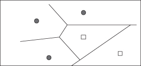
Decision boundaries in 1NN are concatenated segments of the
Voronoi diagram
as shown in Figure
4.28
. The Voronoi diagram decomposes space into Voronoi cells, where each cell consists of all points that are closer to the sample than to other samples. Assume that we have X training samples in a 2-D space. The diagram then partitions the 2-D plane into |X
|
convex polygons, each containing its corresponding sample (and no other), where a convex polygon is a convex region in a 2-D space bounded by lines. For general
k
> 1 case, consider the region in the space for which the set of kNN is the same. This again is a convex polygon and the space is partitioned into convex polygons, within each of which the set of kNN is invariant.

Figure 4.28.
Voronoi diagram in a 2-D space.

The parameter
k
in kNN is often chosen based on experience or knowledge about the classification problem at hand. It is desirable for
k
to be odd to make ties less likely.
k
= 3 and
k
= 5 are common choices, but much larger values up to 100 are also used. An alternative way of setting the parameter is to select
k
through the iterations of testing process, and select
k
that gives best results on testing set.

Time complexity of the algorithm is linear in the size of the training set as we need to compute the distance of each training sample from the new test sample. Of course, the computing time goes up as k goes up, but the advantage is that higher values of k provide smoothing of the classification surface that reduces vulnerability to noise in the training data. At the same time high value for k may destroy the locality of the estimation since farther samples are taken into account, and large k increases the computational burden. In practical applications, typically, k is in units or tens rather than in hundreds or thousands. The nearest neighbor classifier is quite simple algorithm, but very computationally intensive especially in the testing phase. The choice of the distance measure is another important consideration. It is well known that the Euclidean distance measure becomes less discriminating as the number of attributes increases, and in some cases it may be better to use cosine or other measures rather than Euclidean distance.

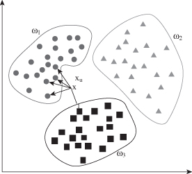
Testing time of the algorithm is independent of the number of classes, and kNN therefore has a potential advantage for classification problems with multiple classes. For the example in Figure
4.29
we have three classes (ω
₁
, ω
₂
, ω
₃
) represented by a set of training samples, and the goal is to find a class label for the testing sample x
_u
. In this case, we use the Euclidean distance and a value of k = 5 neighbors as the threshold. Of the five closest neighbors, four belong to ω
₁
class and 1 belongs to ω
₃
class, so x
_u
is assigned to ω
₁
as the predominant class in the neighborhood.

Figure 4.29.
Nearest neighbor classifier for k = 5.

In summary, kNN classifier only requires a parameter
k
, a set of labeled training samples, and a metric measure for determining distances in an n-dimensional space. kNN classification process is usually based on the following steps:

• Determine parameter k—number of nearest neighbors.
  
• Calculate the distance between each testing sample and all the training samples.
  
• Sort the distance and determine nearest neighbors based on the k-th threshold.
  
• Determine the category (class) for each of the nearest neighbors.
  
• Use simple majority of the category of nearest neighbors as the prediction value of the testing sample classification.
  

There are many techniques available for improving the performance and speed of a nearest neighbor classification. One solution is to choose a subset of the training data for classification. The idea of the
Condensed Nearest Neighbor (CNN)
is to select the smallest subset Z of training data X such that when Z is used instead of X, error in classification of new testing samples does not increase. 1NN is used as the nonparametric estimator for classification. It approximates the classification function in a piecewise linear manner. Only the samples that define the classifier need to be kept. Other samples, inside regions, need not be stored because they belong to the same class. An example of CNN classifier in a 2-D space is given in Figure
4.30
. Greedy CNN algorithm is defined with the following steps:

Figure 4.30.
CNN classifier in a 2-D space.

kNN methodology is relatively simple and could be applicable in many real-world problems. Still, there are some methodological problems such as scalability, “course of dimensionality,” influence of irrelevant attributes, weight factors in the distance measure, and weight factors for votes of k neighbors.

4.7 MODEL SELECTION VERSUS GENERALIZATION

We assume that the empirical data are given according to an unknown probability distribution. The question arises as to whether a finite set of empirical data includes sufficient information such that the underlying regularities can be learned and represented with a corresponding model. A positive answer to this question is a necessary condition for the success of any learning algorithm. A negative answer would yield the consequence that a learning system may remember the empirical data perfectly, and the system may have an unpredictable behavior with unseen data.

We may start discussion about appropriate model selection with an easy problem of learning a Boolean function from examples. Assume that both inputs and outputs are binary. For d inputs, there are 2
^d
different samples, and there are 2
^2d
possible Boolean functions as outputs. Each function is a potential hypothesis h
_i
. In the case of two inputs x
₁
and x
₂
, there are 2
⁴
= 16 different hypotheses as shown in Table
4.1
.

TABLE 4.1.
Boolean Functions as Hypotheses