Data Mining (35 page)
Authors: Mehmed Kantardzic
4.8 MODEL ESTIMATION
A model realized through the data-mining process using different inductive-learning techniques might be estimated using the standard error rate parameter as a measure of its performance. This value expresses an approximation of the true error rate, a parameter defined in SLT. The error rate is computed using a testing data set obtained through one of applied resampling techniques. In addition to the accuracy measured by the error rate, data-mining models can be compared with respect to their speed, robustness, scalability, and interpretability; all these parameters may have an influence on the final verification and validation of the model. In the short overview that follows, we will illustrate the characteristics of the error-rate parameter for classification tasks; similar approaches and analyses are possible for other common data-mining tasks.
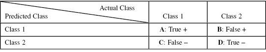
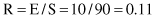
The computation of error rate is based on counting of errors in a testing process. These errors are, for a classification problem, simply defined as misclassification (wrongly classified samples). If all errors are of equal importance, an error rate R is the number of errors E divided by the number of samples S in the testing set:

The accuracy AC of a model is a part of the testing data set that is classified correctly, and it is computed as one minus the error rate:
For standard classification problems, there can be as many as m
2
− m types of errors, where m is the number of classes.
Two tools commonly used to assess the performance of different classification models are the
confusion matrix
and the
lift chart.
A confusion matrix, sometimes called a classification matrix, is used to assess the prediction accuracy of a model. It measures whether a model is confused or not, that is, whether the model is making mistakes in its predictions. The format of a confusion matrix for a two-class case with classes yes and no is shown in Table
4.2
.
TABLE 4.2.
Confusion Matrix for Two-Class Classification Model
If there are only two classes (positive and negative samples, symbolically represented with T and F or with 1 and 0), we can have only two types of errors:
1.
It is expected to be T, but it is classified as F: These are false negative errors (C: False-), and
2.
It is expected to be F, but it is classified as T: These are false positive errors (B: False+).
If there are more than two classes, the types of errors can be summarized in a confusion matrix, as shown in Table
4.3
. For the number of classes m = 3, there are six types of errors (m
2
− m = 3
2
− 3 = 6), and they are represented in bold type in Table
4.3
. Every class contains 30 samples in this example, and the total is 90 testing samples.
TABLE 4.3.
Confusion Matrix for Three Classes
The error rate for this example is
and the corresponding accuracy is

Accuracy is not always the best measure of the quality of the classification model. It is especially true for the real-world problems where the distribution of classes is unbalanced. For example, if the problem is classification of healthy persons from those with the disease. In many cases the medical database for training and testing will contain mostly healthy persons (99%), and only small percentage of people with disease (about 1%). In that case, no matter how good the accuracy of a model is estimated to be, there is no guarantee that it reflects the real world. Therefore, we need other measures for model quality. In practice, several measures are developed, and some of the best known are presented in Table
4.4
. Computation of these measures is based on parameters A, B, C, and D for the confusion matrix in Table
4.2
. Selection of the appropriate measure depends on the application domain, and for example in medical field the most often used are measures: sensitivity and specificity.
TABLE 4.4.
Evaluation Metrics for Confusion Matrix 2 × 2
| Evaluation Metrics | Computation Using Confusion Matrix |
| True positive rate (TP) | TP = A/(A + C) |
| False positive rate (FP) | FP = B/(B + D) |
| Sensitivity (SE) | SE = TP |
| Sensitivity (SP) | SP = 1 − FP |
| Accuracy (AC) | AC = (A + D)/(A + B + C + D) |
| Recall (R) | R = A/(A + B) |
| Precision (P) | P = A/(A + C) |
| F measure (F) | F = 2PR/(P + R) |
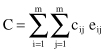
So far we have considered that every error is equally bad. In many data-mining applications, the assumption that all errors have the same weight is unacceptable. So, the differences between various errors should be recorded, and the final measure of the error rate will take into account these differences. When different types of errors are associated with different weights, we need to multiply every error type with the given weight factor c
ij
. If the error elements in the confusion matrix are e
ij
, then the total cost function C (which replaces the number of errors in the accuracy computation) can be calculated as
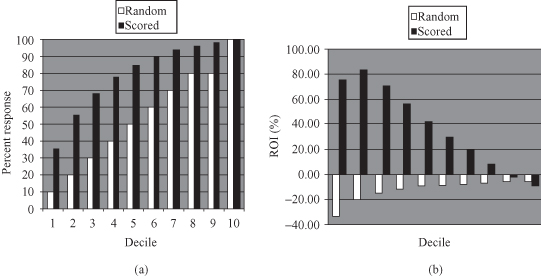
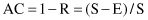
In many data-mining applications, it is not adequate to characterize the performance of a model by a single number that measures the overall error rate. More complex and global measures are necessary to describe the quality of the model. A lift chart, sometimes called a cumulative gains chart, is an additional measure of classification model performance. It shows how classification results are changed by applying the model to different segments of a testing data set. This change ratio, which is hopefully the increase in response rate, is called the “lift.” A lift chart indicates which subset of the dataset contains the greatest possible proportion of positive responses or accurate classification. The higher the lift curve is from the baseline, the better the performance of the model since the baseline represents the null model, which is no model at all. To explain a lift chart, suppose a two-class prediction where the outcomes were yes (a positive response) or no (a negative response). To create a lift chart, instances in the testing dataset are sorted in descending probability order according to the predicted probability of a positive response. When the data are plotted, we can see a graphical depiction of the various probabilities as it is represented with the black histogram in Figure
4.32
a. The baseline, represented as the white histogram on the same figure, indicates the expected result if no model was used at all. Note that the best model is not the one with the highest lift when it is being built with the training data. It is the model that performs the best on unseen, future data.
Figure 4.32.
Assessing the performances of data-mining model. (a) Lift chart; (b) ROI chart.