Data Mining (38 page)

To check the validity of the 383 found patients, 383 randomly chosen patients were mixed with the 383 found previously. Then 150 patients were chosen from the 766 patient samples. An electrophysiologist manually reviewed the 150 patients being blinded to the selection made by the REMIND system. The REMIND system concurred with the manual analysis in 94% (141/150) of the patients. The sensitivity was 99% (69/70) and the specificity was 90% (72/80). Thus it was shown that the REMIND system could fairly accurately identify at-risk patients in a large database. An expert was required to verify the results of the system. Additionally, all of the patients found would be reviewed by a physician before implantation would occur.

From the previous cases we see that a great deal of time was required from experts to prepare data for mining, and careful analysis of a model application needed to take place after deployment. Although applied data-mining techniques (neural and Bayesian networks) will be explained in the following chapters, the emphasis of these stories is on complexity of a data-mining process, and especially deployment phase, in real-world applications. The system developed for Banmedica was measured after analysis in terms of fraudulent cases found and the amount of money saved. If these numbers were not in favor of the system, then it would have been rolled back. In the case of the REMIND system, the results of the system wide search had to be manually analyzed for accuracy. It was not enough that the rules were good, but the actual patients found needed to be reviewed.

4.10 REVIEW QUESTIONS AND PROBLEMS

1. Explain the differences between the basic types of inferences: induction, deduction, and transduction.

2. Why do we use the observational approach in most data-mining tasks?

3. Discuss situations in which we would use the interpolated functions given in Figure
4.3
b,c,d as “the best” data-mining model.

4. Which of the functions have linear parameters and which have nonlinear? Explain why.

5. Explain the difference between interpolation of loss function for classification problems and for regression problems.

6. Is it possible that empirical risk becomes higher than expected risk? Explain.

7. Why is it so difficult to estimate the VC dimension for real-world data-mining applications?

8. What will be the practical benefit of determining the VC dimension in real-world data-mining applications?

9. Classify the common learning tasks explained in Section 4.4 as supervised or unsupervised learning tasks. Explain your classification.

10. Analyze the differences between validation and verification of inductive-based models.

11. In which situations would you recommend the leave-one-out method for validation of data-mining results?

12. Develop a program for generating “fake” data sets using the bootstrap method.

13. Develop a program for plotting an ROC curve based on a table of FAR–FRR results.

14. Develop an algorithm for computing the area below the ROC curve (which is a very important parameter in the evaluation of inductive-learning results for classification problems).

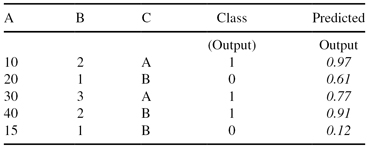
15. The testing data set (inputs: A, B, and C, output: Class) is given together with testing results of the classification (predicted output). Find and plot two points on the ROC curve for the threshold values of 0.5 and 0.8.

16. Machine-learning techniques differ from statistical techniques in that machine learning methods

17. Explain the difference between sensitivity and specificity.

18. When do you need to use a separate validation set, in addition to train and test sets?

19. In this question we will consider learning problems where each instance x is some integer in the set X = {1, 2, … , 127}, and where each hypothesis h
∈
H is an interval of the form a ≤ x ≤ b, where a and b can be any integers between 1 and 127 (inclusive), so long as a ≤ b. A hypothesis a ≤ x ≤ b labels instance x positive if x falls into the interval defined by a and b, and labels the instance negative otherwise. Assume throughout this question that the teacher is only interested in teaching concepts that can be represented by some hypothesis in H.

20. Is it true that the SVM learning algorithm is guaranteed to find the globally optimal hypothesis with respect to its object function? Discuss your answer.

4.11 REFERENCES FOR FURTHER STUDY

Alpaydin, A,
Introduction to Machine Learning
, 2nd edition, The MIT Press, Boston, 2010.

The goal of machine learning is to program computers to use example data or past experience to solve a given problem. Many successful applications of machine learning exist already, including systems that analyze past sales data to predict customer behavior, optimize robot behavior so that a task can be completed using minimum resources, and extract knowledge from bioinformatics data.
Introduction to Machine Learning
is a comprehensive textbook on the subject, covering a broad array of topics not usually included in introductory machine-learning texts. In order to present a unified treatment of machine-learning problems and solutions, it discusses many methods from different fields, including statistics, pattern recognition, neural networks, artificial intelligence, signal processing, control, and data mining. All learning algorithms are explained so that the student can easily move from the equations in the book to a computer program.

Berthold, M., D. J. Hand, eds.,
Intelligent Data Analysis—An Introduction
, Springer, Berlin, Germany, 1999.

The book is a detailed, introductory presentation of the key classes of intelligent data-analysis methods including all common data-mining techniques. The first half of the book is devoted to the discussion of classical statistical issues, ranging from basic concepts of probability and inference to advanced multivariate analyses and Bayesian methods. The second part of the book covers theoretical explanations of data-mining techniques that have their roots in disciplines other than statistics. Numerous illustrations and examples enhance the readers’ knowledge about theory and practical evaluations of data-mining techniques.

Cherkassky, V., F. Mulier,
Learning from Data: Concepts, Theory and Methods
, 2nd edition, John Wiley, New York, 2007.

The book provides a unified treatment of the principles and methods for learning dependencies from data. It establishes a general conceptual framework in which various learning methods from statistics, machine learning, and other disciplines can be applied—showing that a few fundamental principles underlie most new methods being proposed today. An additional strength of this primarily theoretical book is the large number of case studies and examples that simplify and make understandable concepts in SLT.

Engel, A., C. Van den Broeck,
Statistical Mechanics of Learning
, Cambridge University Press, Cambridge, UK, 2001.

The subject of this book is the contribution of machine learning over the last decade by researchers applying the techniques of statistical mechanics. The authors provide a coherent account of various important concepts and techniques that are currently only found scattered in papers. They include many examples and exercises, making this a book that can be used with courses, or for self-teaching, or as a handy reference.

Haykin, S.,
Neural Networks: A Comprehensive Foundation
, Prentice Hall, Upper Saddle River, NJ, 1999.

The book provides a comprehensive foundation for the study of artificial neural networks, recognizing the multidisciplinary nature of the subject. The introductory part explains the basic principles of SLT and the concept of VC dimension. The main part of the book classifies and explains artificial neural networks as learning machines with and without a teacher. The material presented in the book is supported with a large number of examples, problems, and computer-oriented experiments.

Chapter Objectives

• Explain methods of statistical inference commonly used in data-mining applications.
  
• Identify different statistical parameters for assessing differences in data sets.
  
• Describe the components and the basic principles of Naïve Bayesian classifier and the logistic regression method.
  
• Introduce log-linear models using correspondence analysis of contingency tables.
  
• Discuss the concepts of analysis of variance (ANOVA) and linear discriminant analysis (LDA) of multidimensional samples.
  

Statistics is the science of collecting and organizing data and drawing conclusions from data sets. The organization and description of the general characteristics of data sets is the subject area of
descriptive statistics
. How to draw conclusions from data is the subject of
statistical inference
. In this chapter, the emphasis is on the basic principles of statistical inference; other related topics will be described briefly enough to understand the basic concepts.

Statistical data analysis is the most well-established set of methodologies for data mining. Historically, the first computer-based applications of data analysis were developed with the support of statisticians. Ranging from one-dimensional data analysis to multivariate data analysis, statistics offered a variety of methods for data mining, including different types of regression and discriminant analysis. In this short overview of statistical methods that support the data-mining process, we will not cover all approaches and methodologies; a selection has been made of the techniques used most often in real-world data-mining applications.

5.1 STATISTICAL INFERENCE

The totality of the observations with which we are concerned in statistical analysis, whether their number is finite or infinite, constitutes what we call a
population
. The term refers to anything of statistical interest, whether it is a group of people, objects, or events. The number of observations in the population is defined as the size of the population. In general, populations may be finite or infinite, but some finite populations are so large that, in theory, we assume them to be infinite.

In the field of statistical inference, we are interested in arriving at conclusions concerning a population when it is impossible or impractical to observe the entire set of observations that make up the population. For example, in attempting to determine the average length of the life of a certain brand of light bulbs, it would be practically impossible to test all such bulbs. Therefore, we must depend on a subset of observations from the population for most statistical-analysis applications. In statistics, a subset of a population is called a
sample
and it describes a finite data set of n-dimensional vectors. Throughout this book, we will simply call this subset of population
data set
, to eliminate confusion between the two definitions of sample: one (explained earlier) denoting the description of a single entity in the population, and the other (given here) referring to the subset of a population. From a given data set, we build a statistical model of the population that will help us to make inferences concerning that same population. If our inferences from the data set are to be valid, we must obtain samples that are representative of the population. Very often, we are tempted to choose a data set by selecting the most convenient members of the population. But such an approach may lead to erroneous inferences concerning the population. Any sampling procedure that produces inferences that consistently overestimate or underestimate some characteristics of the population is said to be biased. To eliminate any possibility of bias in the sampling procedure, it is desirable to choose a random data set in the sense that the observations are made independently and at random. The main purpose of selecting random samples is to elicit information about unknown population parameters.

The relation between data sets and the system they describe may be used for inductive reasoning: from observed data to knowledge of a (partially) unknown system. Statistical inference is the main form of reasoning relevant to data analysis. The theory of statistical inference consists of those methods by which one makes inferences or generalizations about a population. These methods may be categorized into two major areas:
estimation
and
tests of hypotheses
.

In
estimation,
one wants to come up with a plausible value or a range of plausible values for the unknown parameters of the system. The goal is to gain information from a data set T in order to estimate one or more parameters w belonging to the model of the real-world system f(X, w). A data set T is described by the ordered n-tuples of values for variables: X = {X
₁
, X
₂
, … , X
_n
} (attributes of entities in population):

It can be organized in a tabular form as a set of samples with its corresponding feature values. Once the parameters of the model are estimated, we can use them to make predictions about the random variable Y from the initial set of attributes Y∈ X, based on other variables or sets of variables X* = X − Y. If Y is numeric, we speak about
regression
, and if it takes its values from a discrete, unordered data set, we speak about
classification
.

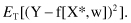
Once we have obtained estimates for the model parameters w from some data set T, we may use the resulting model (analytically given as a function f[X*, w]) to make predictions about Y when we know the corresponding value of the vector X*. The difference between the prediction f(X*, w) and the real value Y is called the prediction error. It should preferably take values close to 0. A natural quality measure of a model f(X*, w), as a predictor of Y, is the expected mean-squared error for the entire data set T:

In
statistical testing
, on the other hand, one has to decide whether a hypothesis concerning the value of the population characteristic should be accepted or rejected in light of an analysis of the data set. A statistical hypothesis is an assertion or conjecture concerning one or more populations. The truth or falsity of a statistical hypothesis can never be known with absolute certainty, unless we examine the entire population. This, of course, would be impractical in most situations, sometimes even impossible. Instead, we test a hypothesis on a randomly selected data set. Evidence from the data set that is inconsistent with the stated hypothesis leads to a rejection of the hypothesis, whereas evidence supporting the hypothesis leads to its acceptance, or more precisely, it implies that the data do not contain sufficient evidence to refute it. The structure of hypothesis testing is formulated with the use of the term
null hypothesis
. This refers to any hypothesis that we wish to test and is denoted by H
₀
. H
₀
is only rejected if the given data set, on the basis of the applied statistical tests, contains strong evidence that the hypothesis is not true. The rejection of H
₀
leads to the acceptance of an alternative hypothesis about the population.

In this chapter, some statistical estimation and hypothesis-testing methods are described in great detail. These methods have been selected primarily based on the applicability of the technique in a data-mining process on a large data set.

5.2 ASSESSING DIFFERENCES IN DATA SETS

For many data-mining tasks, it would be useful to learn the more general characteristics about the given data set, regarding both central tendency and data dispersion. These simple parameters of data sets are obvious descriptors for assessing differences between different data sets. Typical measures of central tendency include
mean
,
median
, and
mode
, while measures of data dispersion include
variance
and
standard deviation
.

The most common and effective numeric measure of the center of the data set is the
mean
value (also called the arithmetic mean). For the set of n numeric values x
₁
, x
₂
, … , x
_n
, for the given feature X, the mean is

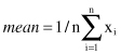
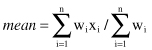
and it is a built-in function (like all other descriptive statistical measures) in most modern, statistical software tools. For each numeric feature in the n-dimensional set of samples, it is possible to calculate the mean value as a central tendency characteristic for this feature. Sometimes, each value x
_i
in a set may be associated with a weight w
_i
, which reflects the frequency of occurrence, significance, or importance attached to the value. In this case, the weighted arithmetic mean or the weighted average value is

Although the mean is the most useful quantity that we use to describe a set of data, it is not the only one. For skewed data sets, a better measure of the center of data is the
median
. It is the middle value of the ordered set of feature values if the set consists of an odd number of elements and it is the average of the middle two values if the number of elements in the set is even. If x
₁
, x
₂
, … , x
_n
represents a data set of size n, arranged in increasing order of magnitude, then the median is defined by