Data Mining (40 page)
Authors: Mehmed Kantardzic
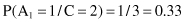
Figure 5.3.
Scatter plots showing the correlation between features from −1 to 1.
These visualization processes are part of the data-understanding phase, and they are essential in preparing better for data mining. This human interpretation helps to obtain a general view of the data. It is also possible to identify abnormal or interesting characteristics, such as anomalies.
5.3 BAYESIAN INFERENCE
It is not hard to imagine situations in which the data are not the only available source of information about the population or about the system to be modeled. The Bayesian method provides a principled way to incorporate this external information into the data-analysis process. This process starts with an already given probability distribution for the analyzed data set. As this distribution is given before any data is considered, it is called a
prior distribution
. The new data set updates this prior distribution into a
posterior distribution
. The basic tool for this updating is the Bayes theorem.
The Bayes theorem represents a theoretical background for a statistical approach to inductive-inferencing classification problems. We will explain first the basic concepts defined in the Bayes theorem, and then, use this theorem in the explanation of the Naïve Bayesian classification process, or the
simple Bayesian classifier
.
Let X be a data sample whose class label is unknown. Let H be some hypothesis: such that the data sample X belongs to a specific class C. We want to determine P(H/X), the probability that the hypothesis H holds given the observed data sample X. P(H/X) is the posterior probability representing our confidence in the hypothesis after X is given. In contrast, P(H) is the prior probability of H for any sample, regardless of how the data in the sample look. The posterior probability P(H/X) is based on more information then the prior probability P(H). The Bayesian theorem provides a way of calculating the posterior probability P(H/X) using probabilities P(H), P(X), and P(X/H). The basic relation is

Suppose now that there is a set of m samples S = {S
1
, S
2
, … , S
m
} (the training data set) where every sample S
i
is represented as an n-dimensional vector {x
1
, x
2
, … , x
n
}. Values x
i
correspond to attributes A
1
, A
2
, … , A
n
, respectively. Also, there are k classes C
1
, C
2
, … , C
k
, and every sample belongs to one of these classes. Given an additional data sample X (its class is unknown), it is possible to predict the class for X using the highest conditional probability P(C
i
/X), where i = 1, … , k. That is the basic idea of Naïve Bayesian classifier. These probabilities are computed using Bayes theorem:

As P(X) is constant for all classes, only the product P(X/C
i
) · P(C
i
) needs to be maximized. We compute the prior probabilities of the class as

where m is total number of training samples.
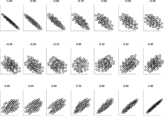
Because the computation of P(X/C
i
) is extremely complex, especially for large data sets, the naïve assumption of conditional independence between attributes is made. Using this assumption, we can express P(X/C
i
) as a product:
where x
t
are values for attributes in the sample X. The probabilities P(x
t
/C
i
) can be estimated from the training data set.
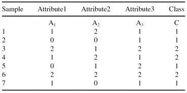
A simple example will show that the Naïve Bayesian classification is a computationally simple process even for large training data sets. Given a training data set of seven four-dimensional samples (Table
5.1
), it is necessary to predict classification of the new sample X = {1, 2, 2, class = ?}. For each sample, A
1
, A
2
, and A
3
are input dimensions and C is the output classification.
TABLE 5.1.
Training Data Set for a Classification Using Naïve Bayesian Classifier
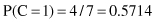
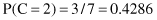
In our example, we need to maximize the product P(X/C
i
) · P(C
i
) for i = 1,2 because there are only two classes. First, we compute prior probabilities P(C
i
) of the class:
Second, we compute conditional probabilities P(x
t
/C
i
) for every attribute value given in the new sample X = {1, 2, 2, C = ?}, (or more precisely, X = {A
1
= 1, A
2
= 2, A
3
= 2, C = ?}) using training data sets: