Data Mining (96 page)

The maximum number of links in the graph is defined by the number of nodes. Since there are k nodes in the graph, and if we exclude the loops as links, there are k(k − 1)/2 possible links that could be presented in the graph. If all links are present, then all nodes are adjacent, and the graph is said to be complete. Consider now what proportion of these links is actually present. The density of a graph is the proportion of actual links in the graph compared with the maximum possible number of links. The density of a graph goes from 0, when there are no links in a graph, to 1, when all possible links are presented.

We can also analyze the paths between a pair of nodes, and they are represented by multiple links. We define a path from s ∈ N to t ∈ N as an alternating sequence of nodes and links, beginning with node s and ending with node t, such that each link connects its preceding with its succeeding node. It is likely that there are several paths between a given pair of nodes, and that these paths are differ in lengths (number of links included in the path). The shortest path between two nodes is referred to as a
geodesic
. The geodesic distance d
_G
or simply the distance between two nodes is defined as the length of a geodesic between them, and it represents the length of the shortest path. By definition, d
_G
(s; s) = 0 for every node s ∈ N, and d
_G
(s; t) = d
_G
(t; s) for each pair of nodes s, t ∈ V. For example, the paths between nodes A and D in Figure
12.2
a are A-B-D and A-B-C-D. The shortest one is A-B-D, and therefore the distance d(A,D) = 2. If there is no path between two nodes, then the distance is infinite (or undefined). The
diameter
of a connected graph is the length of the largest geodesic between any pairs of nodes. It represents the largest nodal eccentricity. The diameter of a graph can range from 1, if the graph is complete, to a maximum of k − 1. If a graph is not connected, its diameter is infinite. For the graph in Figure
12.2
a the diameter is 2.

These basic definitions are introduced for non-labeled and nondirected graphs such as the one in Figure
12.2
a. A
directed graph
, or digraph G(N, L) consists of a set of nodes N and a set of directed links L. Each link is defined by an order pair of nodes (sender, receiver). Since each link is directed, there are k(k − 1) possible links in the graph. A
labeled graph
is a graph in which each link carries some value. Therefore, a labeled graph G consists of three sets of information: G(N,L,V), where the new component V = {v
₁
, v
₂
, … , v
_t
} is a set of values attached to links. An example of a directed graph is given in Figure
12.2
b, while the graph in Figure
12.2
c is a labeled graph. Different applications use different types of graphs in modeling linked data. In this chapter the primary focus is on undirected and unlabeled graphs although the reader still has to be aware that there are numerous graph-mining algorithms for directed and/or labeled graphs.

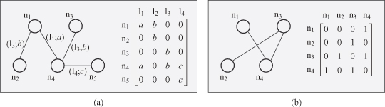
Besides a graphical representation, each graph may be presented in the form of the
incidence matrix
I(G) where nodes are indexing rows and links are indexing columns. The matrix entry in the position (i,j) has value
a
if node n
_i
is incident with
a
, the link l
_j
. The other matrix representation of a graph (in the case of undirected and unlabeled graphs) is the k × k adjacency matrix, where both rows and columns are defined by nodes. The graph-structured data can be transformed without much computational effort into an
adjacency matrix
, which is a well-known representation of a graph in mathematical graph theory. On the intersection (i,j) is the value of 1 if the nodes n
_i
and n
_j
are connected by a link; otherwise it is 0 value (Fig.
12.4
).

Figure 12.4.
Matrix representations of graphs. (a) Incidence matrix:nodes × links; (b) adjancency matrix:nodes ×nodes.

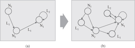
If a graph has labeled links, the following conversion of the graph to a new graph that has labels at its nodes only is applied. This transformation reduces the ambiguity in the adjacency matrix representation. Given a node pair (
u
,
v
) and a directed or undirected link {
u, v
} between the nodes, that is,
node
(
u
)−
link
({
u, v
})−
node
(
v
) where
node
() and
link
() stand for the labels of a node and a link, respectively. The
link
() label information can be removed and transformed into a new
node
(
u, v
), and the following triangular graph may be deduced where the original information of the node pair and the link between them are preserved.

This operation on each link in the original graph can convert the graph into another graph representation having no labels on the links while preserving the topological information of the original graph.

Accordingly, the adjacency matrix of Figure
12.5
a is converted to that of Figure
12.5
b as follows.

Figure 12.5.
Preprocessing of labeled links and self-looped nodes in a graph.

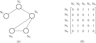
The aforementioned explanation was for directed graphs. But the identical preprocessing may be applied to undirected graphs. The difference from the case of directed graphs is that the adjacency matrix becomes diagonally symmetric. The adjacency matrix of Figure
12.6
a is represented in Figure
12.6
b.

Figure 12.6.
Undirected graph representations.

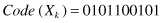
For the sake not only of efficiency in memory consumption but also of efficiency in computations with graphs, we define a code representation of an adjacency matrix as follows. In the case of an undirected graph, the code of an adjacency matrix
X
_k
, that is,
code
(
X
_k
), is represented by a binary number. It is obtained by scanning the upper triangular elements of the matrix along each column until diagonal elements (for an undirected graph). For example, the code of the adjacency matrix in Figure
12.6
b is given by

A variety of operations is defined in graph theory, and corresponding algorithms are developed to efficiently perform these operations. The algorithms work with graphical, matrix, or code representations of graphs. One of the very important operations is the joining of two graphs to form a new, more complex graph. This operation is used in many graph-mining algorithms, including frequent-pattern mining in graphs. The join operation is demonstrated through the example depicted in Figure
12.7
. The examples of the adjacency matrices X
₄
, Y
₄
, and Z
₅
are given in (d) representing the graphs at (a), (b), and (c).

Figure 12.7.
An example of join operation between graphs (a) and (b).