Data Mining (97 page)
Authors: Mehmed Kantardzic
Graph analysis includes a number of parameters that describe the important characteristics of a graph, and they are used as fundamental concepts in developing graphmining algorithms. Over the years, graph-mining researchers have introduced a large number of
centrality indices
, measures of the importance of the nodes in a graph according to one criterion or another.
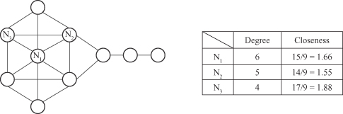
Perhaps the simplest centrality measure is
degree
, which is the number of links for a given node. Degree is a measure in some sense of the “popularity” of a node in the presented graph. Nodes with a high degree are considered to be more central. However, this weights a node only by its immediate neighbors and not by, for example, its two-hop and three-hop neighbors. A more sophisticated centrality measure is
closeness
, which is the mean geodesic (i.e., shortest path) distance between a vertex and all other vertices reachable from it. Examples of computations for both measures are given in Figure
12.8
. Closeness can be regarded as a measure of how long it will take for information to spread from a given node to others in the graph. Nodes that have a low distance to all other nodes in the graph have high closeness centrality.
Figure 12.8.
Degree and closeness parameters of the graph.
Another important class of centrality measures is the class of
betweenness
measures. Betweenness is a measure of the extent to which a vertex lies on the paths between others. The simplest and most widely used betweenness measure is
shortest path betweenness
, or simply
betweenness
. The betweenness of a node
i
is defined to be the fraction of shortest paths between any pair of vertices in a graph that passes through node
i.
This is, in some sense, a measure of the influence a node has over the spread of connections through the network. Nodes with high betweenness values occur on a larger number of shortest paths and are presumably more important than nodes with low betweenness. The parameter is costly to compute especially when the graphs are complex with a large number of nodes and links. Currently, the fastest known algorithms require O(n
3
) time complexity and O(n
2
) space complexity, where n is the number of nodes in the graph.
Illustrative examples of centrality measures and their interpretations are given in Figure
12.9
. Node
X
has importance because it bridges the structural hole between the two clusters of interconnected nodes. It has the highest betweenness measure compared with all the other nodes in the graph. Such nodes get lots of brokerage opportunities and can control the flow in the paths between subgraphs. On the other hand, node
Y
is in the middle of a dense web of nodes that provides easy, short path access to neighboring nodes; thus,
Y
also has a good central position in the subgraph. This characteristic of the node Y is described with the highest degree measure.
Figure 12.9.
Different types of a node’s importance in a graph.

The vertex-betweenness index reflects the amount of control exerted by a given vertex over the interactions between the other vertices in the graph. The other approach to measure betweenness is to concentrate on links in the graph instead of nodes. Edge-betweenness centrality is related to the frequency of an edge placed on the shortest paths between all pairs of vertices. The betweenness centrality of an edge in a network is given by the sum of the edge-betweenness values for all pairs of nodes in the graph going through the given edge. The edges with highest betweenness values are most likely to lie between subgraphs, rather than inside a subgraph. Consequently, successively removing edges with the highest edge-betweenness will eventually isolate subgraphs consisting of nodes that share connections only with other nodes in the same subgraph. This gives the edge-betweenness index a central role in graph-clustering algorithms where it is necessary to separate a large graph into smaller highly connected subgraphs. Edge- (also called link-) betweenness centrality is traditionally determined in two steps:
1.
Compute the length and number of shortest paths between all pairs of nodes through the link.
2.
Sum all link dependencies.
The overall betweenness centrality of a link
v
is obtained by summing up its partial betweenness values for this link, calculated using the graph transformation on breadth first strategy from each node. For example, at the beginning it is given a graph in Figure
12.10
a and it is necessary to find link betweenness measures for all links in the graph. In the first step, we build a “modified” graph that starts with node A, and specifies all links in the graph, layer by layer: first neighbors, second neighbors, and so on. The resulting graph is given in Figure
12.10
b. This graph is the starting point for
partial
betweenness computation. The total betweeness will be the sum of partial scores obtained for transformed graphs with root nodes A to K. The process with each transformed graph in (b) consists of a forward phase and a backward phase, and will be illustrated with activities on the graph in Figure
12.10
b. In the forward phase, the count of shortest paths from A to all other nodes of the network is determined. The computation is performed iteratively, layer by layer. For example, the number of shortest paths from the initial node A to the node I is computed based on the number of shortest paths from node A to the nodes F and G.
Figure 12.10.
Preparatory phase for link-betweenness computation. (a) Initial graph; (b) transformed graph with the root in node A.

The result of the completed forward phase is given in Figure
12.11
a. Each node is labeled with the number of shortest paths from the root node A. For example, the node J has three shortest paths, two of them through the node H (ADHJ and AEHJ) and one through the node G (ADGJ).
Figure 12.11.
Computation of the partial link-betweenness measure. (a) Forward phase; (b) backward phase.
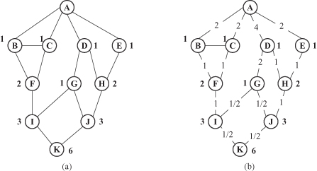
The backward phase starts from the bottom of the layered graph structure, in our example, from node K. If there are multiple paths from the given node up, count betweenness measure of each link fractionally. The proportion is determined by the number of shortest paths to these nodes on the previous layer. What is the amount we are splitting between these links? The amount is defined as
1
+
sum of all betweenness measures entering into the node from below
. For example, from node K there are two paths toward nodes I and J, and because both nodes have the same number of shortest paths (3), the amount we are splitting is 1 + 0 = 1, and the partial betweenness measure for links IK and JK is 0.5. In a similar way, we may compute betweennes measures for node G. Total betweenness value for splitting is 1 + 0.5 + 0.5 = 2. There is only one node up; it is D, and the link-betweenness measure for GD is 2.
When we compute betweenness measures for all links in the graph, the procedure should be repeated for the other nodes in the graph, such as the root nodes, until each node of the network is explored. Finally, all partial link scores determined for different graphs should be added to determine the final link-betweenness score.
Graph-mining applications are far more challenging to implement because of the additional constraints that arise from the structural nature of the underlying graph. The problem of frequent pattern mining has been widely studied in the context of mining transactional data. Recently, the techniques for frequent-pattern mining have also been extended to the case of graph data. This algorithm attempts to find interesting or commonly occurring subgraphs in a set of graphs. Discovery of these patterns may be the sole purpose of the systems, or the discovered patterns may be used for graph classification or graph summarization. The main difference in the case of graphs is that the process of determining support is quite different. The problem can be defined in different ways, depending upon the application domain. In the first case, we have a group of graphs, and we wish to determine all the patterns that support a fraction of the corresponding graphs. In the second case, we have a single large graph, and we wish to determine all the patterns that are supported at least a certain number of times in this large graph. In both cases, we need to account for the isomorphism issue in determining whether one graph is supported by another or not. However, the problem of defining the support is much more challenging if overlaps are allowed between different embeddings. Frequently occurring subgraphs in a large graph or a set of graphs could represent important motifs in the real-world data.
Apriori
-style algorithms can be extended to the case of discovering frequent subgraphs in graph data, by using a similar level-wise strategy of generating (k + 1) candidates from k-patterns. Various measures to mine substructure frequencies in graphs are used similarly in conventional data mining. The selection of the measures depends on the objective and the constraints of the mining approach. The most popular measure in graph-based data mining is a “support” parameter whose definition is identical with that of market-basket analysis. Given a graph data set D, the support of the subgraph Gs, sup(G
s
), is defined as
