Data Mining (94 page)
Authors: Mehmed Kantardzic
Figure 11.8.
Singular value decomposition of initial data.
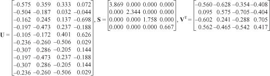
With this initial step, we have already reduced the number of dimensions representing each document from 10 to four. We now show how one would go about further reducing the number of dimensions. When the data set contains many documents, the previous step is not enough to reduce the number of dimensions meaningfully. To perform further reduction, we first observe that matrix
S
provides us with a diagonal matrix of eigenvalues in descending order as follows: λ
1
, … , λ
4
= {3.869, 2.344, 1.758, 0.667}. We will be able to capture most of the variability of the data by retaining only the first k eigenvalues rather than all n terms (in our matrix S, n = 4). If for example k = 2, then we retain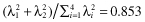 or 85% of the variability when we move from the four new dimensions per document to only two. The rank 2 approximations can be seen in Figure
11.9
. This rank 2 approximation is achieved by selecting the first k columns from
U
, the upper left k × k matrix from
S,
and the top k rows from
V
T
as shown in Figure
11.9
.
Figure 11.9.
Rank 2 approximation of the singular value decomposition.
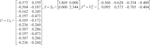
The rank k approximation to
V
T
gives us our dimensionally reduced data set where each document is now described with only two dimensions.
V
T
can be thought of as a transformation of the original document matrix and can be used for any of a number of text-mining tasks, such as classification and clustering. Improved results may be obtained using the newly derived dimensions, comparing against the data-mining tasks using the original word counts.
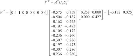
In most text-mining cases, all training documents (in our case 4) would have been included in matrix A and transformed together. Document five (d
5
) was intentionally left out of these calculations to demonstrate a technique called “folding-in,” which allows for a small number of documents to be transformed into the new reduced space and compared with a training document database. Matrices from our previous SVD calculations are used for this transformation. This is done using the following modified formula: . This equation is a rearrangement of terms from the initial SVD equation replacing the original data set, matrix A, with the term counts for document five (d
5
) as matrix A’. The resulting multiplication can be seen in Figure
11.10
. The result is the document d
5
represented in the reduced 2-D space, d
5
= [−0.172, 0.025].
Figure 11.10.
SVD calculations to produce a 2-D approximation for d
5
.
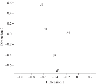
To visualize the transformed data, we have plotted our example documents, d
1..5
, in Figure
11.11
. We now perform the nearest neighbor classification algorithm. If the task is to disambiguate the term “bank,” and the possible classes are “financial institution” and “basketball shot,” then a review of the original text reveals that documents d
1
, d
2
, and d
5
are of the class “financial institution” and documents d
3
and d
4
are of the class “basketball shot.” To classify test document d
5
, we compare d
5
with each other document. The closest neighbor will determine the class of d
5
. Ideally, d
5
should be nearest to d
1
and d
2
, and farthest from d
3
and d
4
, as pointed earlier. Table
11.4
shows these calculations using the Euclidean distance metric. The assessment for which document is closest is made based on both the original 10 dimensions and the reduced set of two dimensions. Table
11.5
shows the same comparison using cosine similarity to compare documents. Cosine similarity is often used in text-mining tasks for document comparisons.
TABLE 11.4.
Use of Euclidean Distance to Find Nearest Neighbor to d
5
in Both 2-d and 10-d (the Smallest Distance Ranks First)
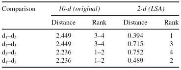
TABLE 11.5.
Use of Cosine Similarity to Find Most Similar Document to d
5
in Both 2-d and 10-d (the Largest Similarity Ranks First)
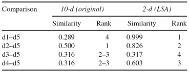
Figure 11.11.
2-D plot of documents and query using LSA.
Euclidean distance as shown in Table
11.4
when using 10 dimensions ranks d
3
and d
4
above d
1
and d
2
. By the formulation of Euclidean distance, when two documents both share a term or both do not share a term, the result is a distance of 0 for that dimension. After applying the LSA transformation, the Euclidean distance ranks d
1
above d
3
and d
4
. However, document d
2
only is ranked above d
3
and not d
4
.
Cosine similarity calculates the cosine of the angle between two vectors representing points in n-dimensional space. The result is a similarity score between 0 and 1, where a 1 shows highest similarity, and 0 shows no similarity. For document vector comparisons, no additional strength of similarity is added by two vectors containing a 0 for a specific term. This is a very beneficial characteristic for textual applications. When we consider Table
11.5
we see that without the transformation, in 10-D space, d
2
is ranked above d
3
and d
4
for containing both terms in d
5
. However, d
1
is ranked below d
3
and d
4
for having more terms than these other sentences. After the LSA transformation, d
1
and d
2
are ranked above d
3
and d
4
, providing the expected ranking. In this simple example the best results occurred when we first transformed the data using LSA and then used cosine similarity to measure the similarity between initial training documents in a database and a new document for comparison. Using the nearest neighbor classifier, d
5
would be classified correctly as a “financial institution” document using cosine similarity for both the 10-d and 2-d cases or using Euclidean distance for the 2-d case. Euclidean distance in the 10-d case would have classified d
5
incorrectly. If we used k-nearest neighbor with k = 3, then Euclidean distance in the 10-d case would have also incorrectly classified d
5
. Clearly, the LSA transformation affects the results of document comparisons, even in this very simple example. Results are better because LSA enable better representation of a document’s semantics.