Authors: Mehmed Kantardzic
Data Mining (42 page)
where ε
j
’s are errors of regression for each of m given samples. The linear model is called linear because the expected value of y
j
is a linear function: the weighted sum of input values.
Linear regression with one input variable is the simplest form of regression. It models a random variable Y (called a response variable) as a linear function of another random variable X (called a predictor variable). Given n samples or data points of the form (x
1
, y
1
), (x
2
, y
2
), … , (x
n
, y
n
), where x
i
∈X and y
i
∈
Y, linear regression can be expressed as

where α and β are regression coefficients. With the assumption that the variance of Y is a constant, these coefficients can be solved by the method of least squares, which minimizes the error between the actual data points and the estimated line. The residual sum of squares is often called the sum of squares of the errors about the regression line and it is denoted by SSE (sum of squares error):
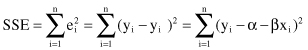
where y
i
is the real output value given in the data set, and y
i
’ is a response value obtained from the model. Differentiating SSE with respect to α and β, we have
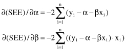
Setting the partial derivatives equal to 0 (minimization of the total error) and rearranging the terms, we obtain the equations
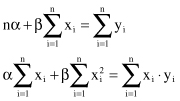
which may be solved simultaneously to yield the computing formulas for α and β. Using standard relations for the mean values, regression coefficients for this simple case of optimization are

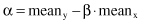
where mean
x
and mean
y
are the mean values for random variables X and Y given in a training data set. It is important to remember that our values of α and β, based on a given data set, are only estimates of the true parameters for the entire population. The equation y = α + βx may be used to predict the mean response y
0
for the given input x
0
, which is not necessarily from the initial set of samples.
For example, if the sample data set is given in the form of a table (Table
5.2
), and we are analyzing the linear regression between two variables (predictor variable A and response variable B), then the linear regression can be expressed as

where α and β coefficients can be calculated based on previous formulas (using mean
A
= 5.4, and mean
B
= 6), and they have the values


TABLE 5.2.
A Database for the Application of Regression Methods
| A | B |
| 1 | 3 |
| 8 | 9 |
| 11 | 11 |
| 4 | 5 |
| 3 | 2 |
The optimal regression line is
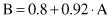
The initial data set and the regression line are graphically represented in Figure
5.4
as a set of points and a corresponding line.
Figure 5.4.
Linear regression for the data set given in Table
5.2
.

Multiple regression
is an extension of linear regression, and involves more than one predictor variable. The response variable Y is modeled as a linear function of several predictor variables. For example, if the predictor attributes are X
1
, X
2
, and X
3
, then the multiple linear regression is expressed as