Read In Pursuit of the Unknown Online
Authors: Ian Stewart
In Pursuit of the Unknown (24 page)
His proof depends on a numerical pattern that was very familiar to Pascal. It is usually called Pascal's triangle, even though he wasn't the first person to notice it. Historians have traced its origins back to the
Chandas Shastra
, a Sanskit text attributed to Pingala, written some time between 500
BC
and 200
BC.
The original has not survived, but the work is known through tenth-century Hindu commentaries. Pascal's triangle looks like this:

where all rows start and end in 1, and each number is the sum of the two immediately above it. We now call these numbers binomial coefficients, because they arise in the algebra of the binomial (two-variable) expression (
p
+
q
)
n
. Namely,
(
p
+
q
)
0
= 1
(
p
+
q
)
1
=
p
+
q
(
p
+
q
)
2
=
p
2
+ 2
pq
+
q
2
(
p
+
q
)
3
=
p
3
+ 3
p
2
q
+ 3
pq
2
+
q
3
(
p
+
q
)
4
=
p
4
+ 4
p
3
q
+ 6
p
2
q
2
+ 4
pq
3
+
q
4
and Pascal's triangle is visible as the coefficients of the separate terms.
Bernoulli's key insight is that if we toss a coin
n
times, with a probability
p
of getting heads, then the probability of a specific number of tosses yielding heads is the corresponding term of (
p
+
q
)
n
, where
q
= 1 â
p
. For example, suppose that I toss the coin three times. Then the eight possible results are:
HHH | Â | Â |
HHT | HTH | THH |
HTT | THT | TTH |
TTT | Â | Â |
where I've grouped the sequences according to the number of heads. So out of the eight possible sequences, there are
1 sequence with 3 heads
3 sequences with 2 heads
3 sequences with 1 heads
1 sequence with 0 heads
The link with binomial coefficients is no coincidence. If you expand the algebraic formula (H + T)
3
but don't collect the terms together, you get
HHH + HHT + HTH + THH + HTT + THT + TTH + TTT
Collecting terms according to the number of Hs then gives
H
3
+ 3H
2
T + 3HT
2
+T
3
After that, it's a matter of replacing each of H and T by its probability,
p or q
respectively.
Even in this case, each extreme HHH and TTT occurs only once in eight trials, and more equitable numbers occur in the other six. A more sophisticated calculation using standard properties of binomial coefficients proves Bernoulli's law of large numbers.
Advances in mathematics often come about because of ignorance. When mathematicians don't know how to calculate something important, they find a way to sneak up on it indirectly. In this case, the problem is to calculate those binomial coefficients. There's an explicit formula, but if, for instance, you want to know the probability of getting exactly 42 heads when tossing a coin 100 times, you have to do 200 multiplications and then simplify a very complicated fraction. (There are short cuts; it's still a big mess.) My computer tells me in a split second that the answer is
28, 258, 808, 871, 162, 574, 166, 368, 460, 400
p
42
q
58
but Bernoulli didn't have that luxury. No one did until the 1960s, and computer algebra systems didn't really become widely available until the late 1980s.
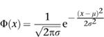
Since this kind of direct calculation wasn't feasible, Bernoulli's immediate successors tried to find good approximations. Around 1730 Abraham De Moivre derived an approximate formula for the probabilities involved in repeated tosses of a biased coin. This led to the error function or normal distribution, often referred to as the âbell curve' because of its shape. What he proved was this. Define the
normal distribution Φ
(
x
) with mean
μ
and variance Ï
2
by the formula
Then for large
n
the probability of getting
m
heads in
n
tosses of a biased coin is very close to Φ(
x
) when
x
=
m/n
â
p
μ =
np
Ï =
npq
Here âmean' refers to the average, and âvariance' is a measure of how far the data spread out â the width of the bell curve. The square root of the variance,
Ï
itself, is called the standard deviation.
Figure 32
(
left
) shows how the value of Φ
x
depends on
x
. The curve looks a bit like a bell, hence the informal name. The bell curve is an example of a probability distribution; this means that the probability of obtaining data between two given values is equal to the area under the curve and between the vertical lines corresponding to those values. The total area under the curve is 1, thanks to that unexpected factor
The idea is most easily grasped using an example.
Figure 32
(
right
) shows a graph of the probabilities of getting various numbers of heads when tossing a fair coin 15 times (rectangular bars) together with the approximating bell curve.
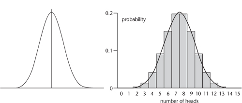
Fig 32
Left
: Bell curve.
right
: How it approximates the number of heads in 15 tosses of a fair coin.
The bell curve began to acquire iconic status when it started showing up in empirical data in the social sciences, not just theoretical mathematics. In 1835 Adolphe Quetelet, a Belgian who among other things pioneered quantitative methods in sociology, collected and analysed large quantities of data on crime, the divorce rate, suicide, births, deaths, human height, weight, and so on â variables that no one expected to conform to any mathematical law, because their underlying causes were too complex and involved human choices. Consider, for example, the emotional torment that drives someone to commit suicide. It seemed ridiculous to think that this could be reduced to a simple formula.
These objections make good sense if you want to predict exactly who will kill themselves, and when. But when Quetelet concentrated on statistical questions, such as the proportion of suicides in various groups of people, various locations, and different years, he started to see patterns. These proved controversial: if you predict that there will be six suicides in Paris next year, how can this make sense when each person involved has free will? They could all change their minds. But the population formed by those who do kill themselves is not specified beforehand; it comes together as a consequence of choices made not just by those who commit suicide, but by those who thought about it and didn't. People exercise free will in the context of many other things, which influence what they freely decide: here the constraints include financial problems, relationship problems, mental state, religious background. . . In any case, the bell curve does not make exact predictions; it just states which figure is most likely. Five or seven suicides might occur, leaving plenty of room for anyone to exercise free will and change their mind.
The data eventually won the day: for whatever reason, people
en masse
behaved more predictably than individuals. Perhaps the simplest example was height. When Quetelet plotted the proportions of people with a given height, he obtained a beautiful bell curve,
Figure 33
. He got the same shape of curve for many other social variables.
Quetelet was so struck by his results that he wrote a book,
Sur l'homme et le développement de ses facultés
(
â
1Treatise on Man and the Development of His Faculties
'
) published in 1835. In it, he introduced the notion of the âaverage man', a fictitious individual who was in every respect average. It has long been noted that this doesn't entirely work: the average âman' â that is, person, so the calculation includes males and females â has (slightly less than) one breast, one testicle, 2.3 children, and so on. Nevertheless Quetelet viewed his average man as the goal of social justice, not just a suggestive mathematical fiction. It's not quite as absurd as it sounds. For example, if human wealth is spread equally to all, then everyone will have average wealth. It's not a practical goal, barring enormous social changes, but someone with strong egalitarian views might defend it as a desirable target.