In Pursuit of the Unknown (25 page)
Read In Pursuit of the Unknown Online
Authors: Ian Stewart
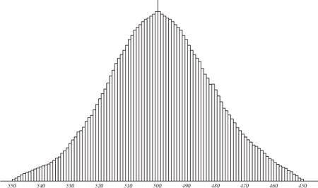
Fig 33
Quetelet's graph of how many people (vertical axis) have a given height (horizontal axis).
The bell curve rapidly became an icon in probability theory, especially its applied arm, statistics. There were two main reasons: the bell curve was relatively simple to calculate, and there was a theoretical reason for it to occur in practice. One of the main sources for this way of thinking was eighteenth-century astronomy. Observational data are subject to errors, caused by slight variations in apparatus, human mistakes, or merely the movement of air currents in the atmosphere. Astronomers of the period wanted to observe planets, comets, and asteroids, and calculate their orbits, and this required finding whichever orbit fitted the data best. The fit would never be perfect.
The practical solution to this problem appeared first. It boiled down to this: run a straight line through the data, and choose this line so that the total error is as small as possible. Errors here have to be considered positive, and the easy way to achieve this while keeping the algebra nice is to square them. So the total error is the sum of the squares of the deviations of observations from the straight line model, and the desired line minimises this. In 1805 the French mathematician Adrien-Marie Legendre discovered a simple formula for this line, making it easy to calculate. The result is called the method of least squares.
Figure 34
illustrates the method on artificial data relating stress (measured by a questionnaire) and blood pressure.
The line in the figure, found using Legendre's formula, fits the data most closely according to the squared-error measure. Within ten years the method of least squares was standard among astronomers in France, Prussia, and Italy. Within another twenty years it was standard in England.
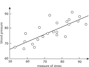
Fig 34
Using the method of least squares to relate blood pressure and stress. Dots: data. Solid line: best-fitting straight line.
Gauss made the method of least squares a cornerstone of his work in celestial mechanics. He got into the area in 1801 by successfully predicting the return of the asteroid Ceres after it was hidden in the glare of the Sun, when most astronomers thought the available data were too limited. This triumph sealed his mathematical reputation among the public and set him up for life as professor of astronomy at the University of Göttingen. Gauss didn't use least squares for this particular prediction: his calculations boiled down to solving an algebraic equation of the eighth degree, which he did by a specially invented numerical method. But in his later work, culminating in his 1809
Theoria Motus Corporum Coelestium in Sectionibus Conicis Solem Ambientum
(âTheory of Motion of the Celestial Bodies Moving in Conic Sections around the Sun') he placed great emphasis on the method of least squares. He also stated that he had developed the idea, and used it, ten years before Legendre, which caused a bit of a fuss. It was very likely true, however, and Gauss's justification of the method was quite different. Legendre had viewed it as an exercise in curve-fitting, whereas Gauss saw it as a way to fit a probability distribution. His justification of the formula assumed that the underlying data, to which the straight line was being fitted, followed a bell curve.
It remained to justify the justification. Why should observational errors be normally distributed? In 1810 Laplace supplied an astonishing answer,
also motivated by astronomy. In many branches of science it is standard to make the same observation several times, independently, and then take the average. So it is natural to model this procedure mathematically. Laplace used the Fourier transform, see
Chapter 9
, to prove that the average of many observations is described by a bell curve, even if the individual observations are not. His result, the central limit theorem, was a major turning point in probability and statistics, because it provided a theoretical justification for using the mathematicians' favourite distribution, the bell curve, in the analysis of observational errors.
3
The central limit theorem singled out the bell curve as the probability distribution uniquely suited to the mean of many repeated observations. It therefore acquired the name ânormal distribution', and was seen as the default choice for a probability distribution. Not only did the normal distribution have pleasant mathematical properties, but there was also a solid reason for assuming it modelled real data. This combination of attributes proved very attractive to scientists wishing to gain insights into the social phenomena that had interested Quetelet, because it offered a way to analyse data from official records. In 1865 Francis Galton studied how a child's height relates to its parents' heights. This was part of a wider goal: understanding heredity â how human characteristics pass from parent to child. Ironically, Laplace's central limit theorem initially led Galton to doubt that this kind of inheritance existed. And, even if it did, proving that would be difficult, because the central limit theorem was a double-edged sword. Quetelet had found a beautiful bell curve for heights, but that seemed to imply very little about the different factors that affected height, because the central limit theorem predicted a normal distribution anyway, whatever the distributions of those factors might be. Even if characteristics of the parents were among those factors, they might be overwhelmed by all the others â such as nutrition, health, social status, and so on.
By 1889, however, Galton had found a way out of this dilemma. The proof of Laplace's wonderful theorem relied on averaging out the effects of many distinct factors, but these had to satisfy some stringent conditions. In 1875 Galton described these conditions as âhighly artificial', and noted that the influences being averaged
must be (1) all independent in their effects, (2) all equal [having the same probability distribution], (3) all admitting of being treated as
simple alternatives âabove average' or âbelow average'; and (4) . . . calculated on the supposition that the variable influences are infinitely numerous.
None of these conditions applied to human heredity. Condition (4) corresponds to Laplace's assumption that the number of factors being added
tends to
infinity, so âinfinitely numerous' is a bit of an exaggeration; however, what the mathematics established was that to get a good approximation to a normal distribution, you had to combine a large number of factors. Each of these contributed a small amount to the average: with, say, a hundred factors, each contributed one hundredth of its value. Galton referred to such factors as âpetty'. Each on its own had no significant effect.
There was a potential way out, and Galton seized on it. The central limit theorem provided a sufficient condition for a distribution to be normal, not a necessary one. Even when its assumptions failed, the distribution concerned might still be normal
for other reasons
. Galton's task was to find out what those reasons might be. To have any hope of linking to heredity, they had to apply to a combination of a few large and disparate influences, not to a huge number of insignificant influences. He slowly groped his way towards a solution, and found it through two experiments, both dating to 1877. One was a device he called a quincunx, in which ball bearings fell down a slope, bouncing off an array of pins, with an equal chance of going left or right. In theory the balls should pile up at the bottom according to a binomial distribution, a discrete approximation to the normal distribution, so they should â and did â form a roughly bellshaped heap, like
Figure 32
(
right
). His key insight was to imagine temporarily halting the balls when they were part way down. They would still form a bell curve, but it would be narrower than the final one. Imagine releasing just one compartment of balls. It would fall to the bottom, spreading out into a tiny bell curve. The same went for any other compartment. And that meant that the final, large bell curve could be viewed as a sum of lots of tiny ones. The bell curve reproduces itself when several factors, each following its own separate bell curve, are combined.
The clincher arrived when Galton bred sweet peas. In 1875 he distributed seeds to seven friends. Each received 70 seeds, but one received very light seeds, one slightly heavier ones, and so on. In 1877 he measured the weights of the seeds of the resulting progeny. Each group was normally distributed, but the mean weight differed in each case, being comparable to the weight of each seed in the original group. When he
combined the data for all of the groups, the results were again normally distributed, but the variance was bigger â the bell curve was wider. Again, this suggested that combining several bell curves led to another bell curve. Galton tracked down the mathematical reason for this. Suppose that two random variables are normally distributed, not necessarily with the same means or the same variances. Then their sum is also normally distributed; its mean is the sum of the two means, and its variance is the sum of the two variances. Obviously the same goes for sums of three, four, or more normally distributed random variables.
This theorem works when a small number of factors are combined, and each factor can be multiplied by a constant, so it actually works for any linear combination. The normal distribution is valid even when the effect of each factor is large. Now Galton could see how this result applied to heredity. Suppose that the random variable given by the height of a child is some combination of the corresponding random variables for the heights of its parents, and these are normally distributed. Assuming that the hereditary factors work by addition, the child's height will also be normally distributed.
Galton wrote his ideas up in 1889 under the title
Natural Inheritance
. In particular, he discussed an idea he called regression. When one tall parent and one short one have children, the mean height of the children should be intermediate â in fact, it should be the average of the parents' heights. The variance likewise should be the average of the variances, but the variances for the parents seemed to be roughly equal, so the variance didn't change much. As successive generations passed, the mean height would âregress' to a fixed middle-of-the-road value, while the variance would stay pretty much unchanged. So Quetelet's neat bell curve could survive from one generation to the next. Its peak would quickly settle to a fixed value, the overall mean, while its width would stay the same. So each generation would have the same diversity of heights, despite regression to the mean. Diversity would be maintained by rare individuals who failed to regress and was self-sustaining in a sufficiently large population.
With the central role of the bell curve firmly cemented to what at the time were considered solid foundations, statisticians could build on Galton's insights and workers in other fields could apply the results. Social science was an early beneficiary, but biology soon followed, and the physical sciences were already ahead of the game thanks to Legendre, Laplace, and Gauss. Soon an entire statistical toolbox was available for anyone who
wanted to extract patterns from data. I'll focus on just one technique, because it is routinely used to determine the efficacy of drugs and medical procedures, along with many other applications. It is called hypothesis testing, and its goal is to assess the significance of apparent patterns in data. It was founded by four people: the Englishmen Ronald Aylmer Fisher, Karl Pearson, and his son Egon, together with a Russian-born Pole who spent most of his life in America, Jerzy Neyman. I'll concentrate on Fisher, who developed the basic ideas when working as an agricultural statistician at Rothamstead Experimental Station, analysing new breeds of plants.