Read In Pursuit of the Unknown Online
Authors: Ian Stewart
In Pursuit of the Unknown (29 page)
The wave equation emerges from Newton's second law of motion if we apply Bernoulli's approach at the level of equations rather than solutions. In 1746 Jean Le Rond d'Alembert followed standard procedure, treating a vibrating violin string as a collection of point masses, but instead of solving the equations and looking for a pattern when the number of masses tended to infinity, he worked out what happened to the equations themselves. He derived an equation that described how the shape of the string changes over time. But before I show you what it looks like, we need a new idea, called a âpartial derivative'.
Imagine yourself in the middle of the ocean, watching waves of various shapes and sizes pass by. As they do so, you bob up and down. Physically, you can describe how your surroundings are changing in several different ways. In particular, you can focus on changes in time or changes in space. As time passes at your location, the rate at which your height changes, with respect to time, is the derivative (in the sense of calculus,
Chapter 3
) of your height, also with respect to time. But this doesn't describe the shape of the ocean near you, just how high the waves are as they pass you. To describe the shape, you can freeze time (conceptually) and work out how high the waves are: not just at your location, but at nearby ones. Then you can use calculus to work out how steeply the wave
slopes
at your location. Are you at a peak or trough? If so, the slope is zero. Are you halfway down the side of a wave? If so, the slope is quite large. In terms of calculus, you can put a number to that slope by working out the derivative of the wave's height with respect to space.
If a function
u
depends on just one variable, call it
x
, we write the derivative as d
u
/d
x:
âsmall change in
u
divided by small change in
x'
. But in the context of ocean waves the function
u
, the wave height, depends not just on space
x
but also on time
t
. At any fixed instant of time, we can still work out d
u
/d
x;
it tells us the local slope of the wave. But instead of fixing
time and letting space vary, we can also fix space and let time vary; this tells us the rate at which we are bobbing up and down. We could use the notation d
u
/d
t
for this âtime derivative' and interpret it as âsmall change in
u
divided by small change in
t'
. But this notation hides an ambiguity: the small change in height,
du
, may be, and usually is, different in the two cases. If you forget that, you are likely to get your sums wrong. When we are differentiating with respect to space, we let the space variable change a little bit and see how the height changes; when we are differentiating with respect to time, we let the time variable change a little bit and see how the height changes. There is no reason why changes over time should equal changes over space.
So mathematicians decided to remind themselves of this ambiguity by changing the symbol d to something that did not (directly) make them think âsmall change'. They settled on a very cute curly d, written
â
. Then they wrote the two derivatives as â
u
/â
x
and â
u
/â
t
. You could argue that this isn't a big advance, because it's just as easy to confuse two different meanings of â
u
. There are two answers to this criticism. One is that in this context you are not supposed to think of â
u
as a specific small change in
u
. The other is that using a fancy new symbol reminds you not to get confused. The second answer definitely works: as soon as you see
â
, it tells you that you will be looking at rates of change with respect to several different variables. These rates of change are called
partial derivatives
, because conceptually you change only part of the set of variables, keeping the rest fixed.
When d'Alembert worked out his equation for the vibrating string, he faced just this situation. The shape of the string depends on space â how far along the string you look â and on time. Newton's second law of motion told him that the acceleration of a small segment of string is proportional to the force that acts on it. Acceleration is a (second) time derivative. But the force is caused by neighbouring segments of the string pulling on the one we're interested in, and âneighbouring' means small changes in
space
. When he calculated those forces, he was led to the equation
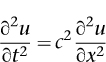
where
u
(
x
,
t
) is the vertical position at location
x
on the string at time
t
, and
c
is a constant related to the tension in the string and how springy it is. The
calculations were actually easier than Bernoulli's, because they avoided introducing special features of particular solutions.
1
D'Alembert's elegant formula is the
wave equation
. Like Newton's second law, it is a differential equation â it involves (second) derivatives of
u
. Since these are partial derivatives, it is a
partial differential equation
. The second space derivative represents the net force acting on the string, and the second time derivative is the acceleration. The wave equation set a precedent: most of the key equations of classical mathematical physics, and a lot of the modern ones for that matter, are partial differential equations.
Once d'Alembert had written down his wave equation, he was in a position to solve it. This task was made much easier because it turned out to be a
linear
equation. Partial differential equations have many solutions, typically infinitely many, because each initial state leads to a distinct solution. For example, the violin string can in principle be bent into any shape you like before it is released and the wave equation takes over. âLinear' means that if
u
(
x
,
t
) and
v
(
x
,
t
) are solutions, then so is any linear combination
au
(
x
,
t
) +
bv
(
x
,
t
), where
a
and
b
are constants. Another term is âsuperposition'. The linearity of the wave equation stems from the approximation that Bernoulli and d'Alembert had to make to get something they could solve: all disturbances are assumed to be small. Now the force exerted by the string can be closely approximated by a linear combination of the displacements of the individual masses. A better approximation would lead to a nonlinear partial differential equation, and life would be far more complicated. In the long run, these complications have to be tackled head-on, but the pioneers had enough to contend with already, so they worked with an approximate but very elegant equation and confined their attention to small-amplitude waves. It worked very well. In fact, it often worked pretty well for waves of larger amplitude too, a lucky bonus.
D'Alembert knew he was on the right track because he found solutions in which a fixed shape travelled along the string, just like a wave.
2
The speed of the wave turned out to be the constant
c
in the equation. The wave could travel either to the left or to the right, and here the superposition principle came into play. D'Alembert proved that every solution is a superposition of two waves, one travelling leftwards and the other rightwards. Moreover, each separate wave could have any shape whatsoever.
3
The standing waves found in the violin string, with fixed ends, turn out to be a combination of two waves of the same shape, one being upside down compared to the other, with one travelling to the left
and the other (upside down) travelling to the right. At the ends, the two waves exactly cancel each other out: peaks of one coincide with troughs of the other. So they comply with the physical boundary conditions.
Mathematicians now had an embarrassment of riches. There were two ways to solve the wave equation: Bernoulli's, which led to sines and cosines, and d'Alembert's, which led to waves with any shape whatsoever. At first it looked as though d'Alembert's solution must be more general: sines and cosines are functions, but most functions are not sines and cosines. However, the wave equation is linear, so you could combine Bernoulli's solutions by adding constant multiples of them together. To keep it simple consider just a snapshot at a fixed time, getting rid of the time-dependence.
Figure 37
shows 5 sin
x +
4 sin
2x â
2 cos
6x
, for example. It has a fairly irregular shape, and it wiggles a lot, but it's still smooth and wavy.
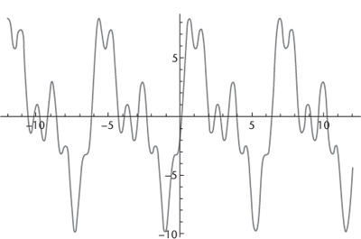
Fig 37
Typical combination of sines and cosines with various amplitudes and frequencies.
What bothered the more thoughtful mathematicians was that some functions are very rough and jagged, and you can't get those as a linear combination of sines and cosines. Well, not if you use finitely many terms â and that suggested a way out. A convergent infinite series of sines and cosines (one whose sum to infinity makes sense) also satisfies the wave equation. Does it allow jagged functions as well as smooth ones? The leading mathematicians argued about this question, which finally came to a head when the same issue turned up in the theory of heat. Problems about heat flow naturally involved discontinuous functions, with sudden
jumps, which was even worse than jagged ones. I'll tell that story in
Chapter 9
, but the upshot is that most âreasonable' wave shapes can be represented by an infinite series of sines and cosines, so they can be approximated as closely as you wish by finite combinations of sines and cosines.
Sines and cosines explain the harmonious ratios that so impressed the Pythagoreans. These special shapes of waves are important in the theory of sound because they represent âpure' tones â single notes on an ideal instrument, so to speak. Any real instrument produces mixtures of pure notes. If you pluck a violin string, the main note you hear is the sin
x
wave, but superposed on that is a bit of sin 2
x
, maybe some sin 3
x
, and so on. The main note is called the fundamental and the others are its harmonics. The number in front of
x
is called the wave number. Bernoulli's calculations tell us that the wave number is proportional to the frequency: how many times the string vibrates, for that particular sine wave, during a single oscillation of the fundamental.
In particular, sin
2x
has twice the frequency of sin
x
. What does it sound like? It is the note
one octave higher
. This is the note that sounds most harmonious when played alongside the fundamental. If you look at the shape of the string for the second mode (sin 2
x
) in
Figure 36
, you'll notice that it crosses the axis at its midpoint as well as the two ends. At that point, a so-called node, it remains fixed. If you placed your finger at that point, the two halves of the string would still be able to vibrate in the sin
2x
pattern, but not in the sin
x
one. This explains the Pythagorean discovery that a string half as long produced a note one octave higher. A similar explanation deals with the other simple ratios that they discovered: they are all associated with sine curves whose frequencies have that ratio, and such curves fit together neatly on a string of fixed length whose ends are not allowed to move.
Why do these ratios sound harmonious? Part of the explanation is that sine waves with frequencies that are not in simple ratios produce an effect called âbeats' when they are superposed. For instance, a ratio like 11 : 23 corresponds to sin 11
x
+ sin 23
x
, which looks like
Figure 38
, with lots of sudden changes in shape. Another part is that the ear responds to incoming sounds in roughly the same way as the violin string. The ear, too, vibrates. When two notes beat, the corresponding sound is like a buzzing noise that repeatedly gets louder and softer. So it doesn't sound harmonious. However, there is a third part of the explanation: the ears of babies become attuned to the sounds that they hear most often. There are more nerve connections from the brain to the ear than there are in the
other direction. So the brain adjusts the ear's response to incoming sounds. In other words, what we consider to be harmonious has a cultural dimension. But the simplest ratios are naturally harmonious, so most cultures use them.