Ancient DNA: Methods and Protocols (46 page)

5. In “Site Models,” select the optimal substitution model for each data partition (see Note 3). If a partition represents an in-frame protein-coding gene, options are available in the 234

S.Y.W. Ho

drop-down menu for partitioning the gene into separate codon positions. The models for the different codon positons can be unlinked by checking the relevant boxes. Users can also implement a model of postmortem DNA damage if desired (see Note 4).

6. In “Clock Models,” the default settings should generally be acceptable. Users have the option of selecting a relaxed molecular-clock model for each data partition (see Note 5).

7. In “Trees,” the demographic model needs to be selected. This will determine the coalescent model to be used in the analysis.

The simplest is “Constant Size,” which has a single parameter describing the effective population size. In addition to simple parametric models, there are several more fl exible models available (see Note 6). Users should repeat the analysis using a number of candidate models, and the results can be compared using Bayes factors (see Note 7).

8. In “Priors” the default settings can be retained unless the user wishes to include a known mutation rate or internal-node calibrations in the analysis. This can be done by choosing the form and parameters of the prior distribution for the mutation rate or for the age of a selected internal node(s) in the tree. For calibrations, a number of options are available and the choice will depend on the nature of the calibrating information (see Note 8).

The internal node(s) should have been defi ned in the “Taxon Sets” tab (see step 2).

9. In “MCMC,” the details of the Markov chain Monte Carlo (MCMC) analysis need to be specifi ed. MCMC is a technique used to estimate the posterior distributions of parameters in the analysis, including the tree topology. The default settings (samples drawn every 1,000 steps over a total of 10,000,000

steps) might suffi ce for relatively simple analyses of small data sets. However, a larger number of steps will normally be

required for analyses involving parameter-rich models and/or larger data sets (see Note 9).

10. Click on “Generate BEAST fi le” to create an XML-formatted input fi le for
BEAST
.

3.2. Bayesian

1. Run
BEAST
using the input fi le produced by
BEAUti
in the
Phylogenetic Analysis

procedure described above. If the data set is very large, it might be necessary to increase the memory allocation (see

Note 10).

2. The output is written to two main fi les. Posterior samples of parameters are written to the “.log” fi le, while posterior samples of trees are written to the “.trees” fi le.

24 Phylogenetic Analysis of Ancient DNA using
BEAST

235

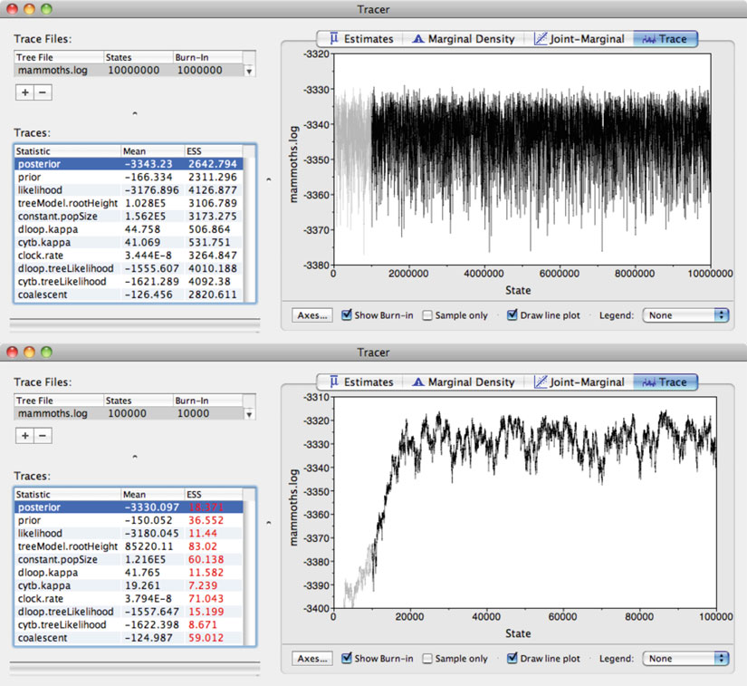
Fig. 3. Screenshot showing examples of trace analyses in the diagnostic software
Tracer
, which is used to process the output from a Bayesian phylogenetic analysis conducted in
BEAST
. In both panels, the fi rst 10% of MCMC samples have been discarded as “burn-in” by default. The upper panel displays a trace plot from an analysis that satisfi es two major diagnostic criteria. First, the plot is approximately horizontal, suggesting convergence to the stationary distribution; however, this needs to be confi rmed by conducting multiple runs. Second, the effective sample size (ESS) values are all greater than 200, indicating suffi cient sampling from the stationary distribution. The lower panel shows an analysis that does not satisfy the two major diagnostic criteria. First, an insuffi cient number of samples have been discarded as burn-in, as indicated by the upward trend in the posterior probability at the beginning of the trace plot. Second, all of the ESS values are well below 200 (shown in
red
), indicating insuffi cient sampling. These problems can be rectifi ed by running the analysis for a greater number of steps and by discarding a larger proportion of the samples as burn-in.

3.3. Processing and

1. Open
Tracer
and import the “.log” fi le.

Interpreting Output

2. Two key aspects of the MCMC analysis need to be checked
(Fig. 3
).

(a)

Convergence of the Markov chain to the stationary distribution is essential. This is suggested by a fl attening of the 236

S.Y.W. Ho

traces of all parameter estimates, but should be confi rmed by conducting replicate
BEAST
analyses and checking that the traces of all replicates converge on the same values.

(b) Acceptable sampling from the stationary distribution is desirable in order to gain reliable estimates of parameter variance. This can be determined through inspection of the effective sample size (ESS) for each parameter (see Note 9).

In general, values above 200 are acceptable, although

higher values are preferable especially for parameters of

interest. It is essential that ESS values for important parameters, such as the likelihood, are greater than 200.

3. If multiple independent MCMC analyses have been performed, the output fi les can be combined using

LogCombiner
. The

diagnostic results from
Tracer
should be consulted to determine the appropriate number of steps to discard as “burn-in.”

4. If one of the fl exible demographic models has been employed (skyline or skyride plot), population history can be plotted in Tracer . This is done by selecting the appropriate option in the “Analysis” menu and opening the corresponding “.trees” fi le.

Tracer
displays the demographic reconstruction in a new window. The raw data for the plot can be exported for further analysis using statistical software or to produce publication-quality fi gures using illustrating software.

5. The “.trees” fi le is processed in two steps.

(a)

Open
TreeAnnotator
and import the “.trees” fi le. The user needs to select a method for summarizing the sampled

trees and for scaling the node heights in the summary tree.

The standard method is to select the tree with the maximum product of clade credibilities and to scale the node

heights to their mean posterior values. The user also needs to select an appropriate number of samples to discard as

burn-in. Note here that the number of
samples
needs to be specifi ed, not the number of
MCMC steps
.

(b) View the
TreeAnnotator
output fi le using a tree-viewing program, such as
FigTree
. For an example, see
Fig. 4 .

24 Phylogenetic Analysis of Ancient DNA using
BEAST

237

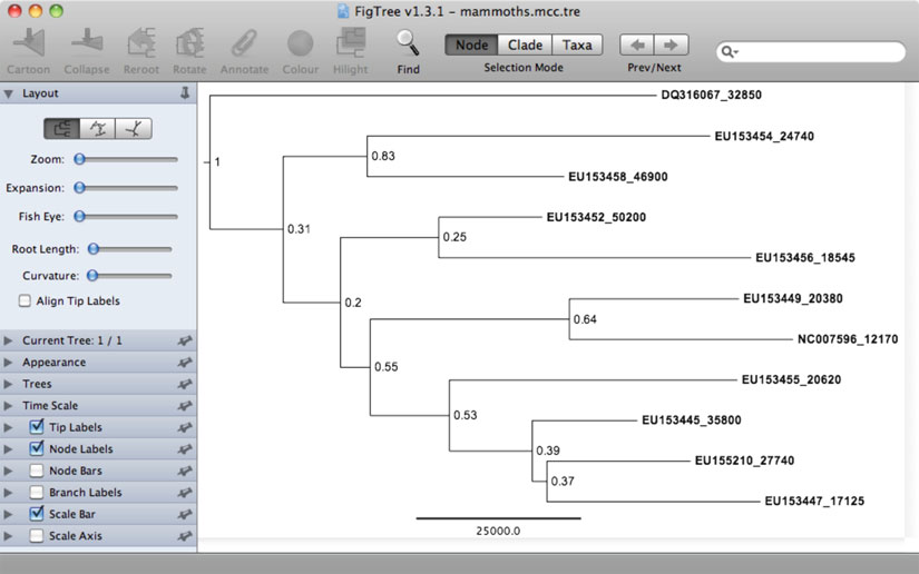
Fig. 4. Screenshot showing a maximum-clade-credibility tree displayed in the tree-viewing software
FigTree
. Internal nodes have been labeled with posterior probabilities. The tree is drawn to a timescale, with the scale bar representing 25,000 years.

4. Notes

1. Sometimes the age of a sample cannot be determined precisely by radiometric or stratigraphic means. For example, a sample might be too old to be dated reliably using radiocarbon techniques, which have an upper limit of around 50,000 years. In these cases, it is possible to treat the age of the sequence as an
estimable parameter in a phylogenetic analysis

( 18 )
. This

approach can be taken if the sampling time is entirely unknown or if one wishes to model uncertainty using a parametric distribution
( 19 )
.

2. The sampling times of the sequences are not always able to provide suffi cient temporal information to calibrate the analysis. This can be investigated using a date-randomization test, which involves repeating the analysis a number of times, with the sequence ages randomly shuffl ed, to generate a null distribution. If the 95% HPDs of the rate estimates from the replicates all exclude the mean posterior estimate from the original data set, the sampling times can be taken as being suffi ciently informative for calibration. This diagnostic approach has been used in a number of studies of aDNA
( 20– 23
) .

238

S.Y.W. Ho

3. The best-fi t model of nucleotide substitution can be selected using various criteria, including the hierarchical likelihood-ratio test, Akaike Information Criterion, and the Bayesian Information Criterion. These can be computed using software such as
Modelgenerator
( 24
) and
ModelTest
( 25
) , which enable the comparison of 56 different time-reversible substitution models. It has been demonstrated that the Bayesian Information Criterion performs well across a range of conditions
( 26 )
.

4. Postmortem damage can be accommodated using an age—

dependent
( 27 )
or age-independent
( 28 )
model of DNA decay.

These models can be applied either to transitional mutations only, or to both transversions and transitions. Empirical studies have shown that postmortem damage is dominated by transitions
( 29, 30
) .

5. Rate heterogeneity among lineages can be modeled using a relaxed molecular clock. The standard approach in

BEAST

involves the uncorrelated lognormal relaxed clock, which assumes that the rates among branches follow a lognormal distribution
( 31
) . The mean and standard deviation of this distribution are estimated in the analysis. The model is termed “uncorrelated”

because it does not involve an
a priori
assumption that rates are correlated between adjacent branches. In some respects, this model is suitable for intraspecifi c data because there is no expectation that rates vary among conspecifi c lineages in an autocorrelated manner
( 32
) . However, a more important consideration relates to whether it is appropriate to use a relaxed-clock model for population-level data at all, given that it is likely to lead to overparameterization. Drummond and Suchard
( 33
) recently introduced random local clocks, which might be more suitable for low-information data sets that do not conform to a strict molecular clock.

6. The demographic history of a species cannot always be satisfac-torily described by a simple parametric model such as exponential or logistic growth. Instead, it is possible to employ a more fl
exible model such as the Bayesian skyline ( 34 )
or Bayesian skyride
( 35
) . Although these methods still involve the typical coalescent assumptions of random mating and selective neutrality, they allow changes in population size to be reconstructed from the sequence data. The skyline and skyride methods can be chosen in
BEAUti
and demographic plots can be generated in
Tracer
. For a recent review of these methods, see Ho and Shapiro
( 36 )
.

7. Bayesian model selection can be performed by calculating Bayes factors. The Bayes factor represents the support for one model over another, and can be calculated in
Tracer
. First, a 24 Phylogenetic Analysis of Ancient DNA using
BEAST

239

separate analysis needs to be performed using each of the models to be compared. The “.log” fi les are then opened in
Tracer
, which can be used to compute the Bayes factor for each pairwise comparison. The method used to calculate the Bayes factor, which involves computation of the harmonic mean of the log likelihood
( 37 )
, has been deprecated on statistical grounds
( 38, 39
) . Better methods for computing Bayes factors have been developed, but are not yet available in
Tracer
.

8. In some cases, independent calibrating information might be available for at least one internal node in the tree. For example, the fossil record might be able to provide an estimate of the age of the root. This calibrating information can be incorporated in the form of a prior distribution for the age of the node.

Several distributions are available; the choice among these should be determined by the nature of the calibration and its associated uncertainty
( 19,
40, 41
) .