Authors: Mehmed Kantardzic
Data Mining (116 page)
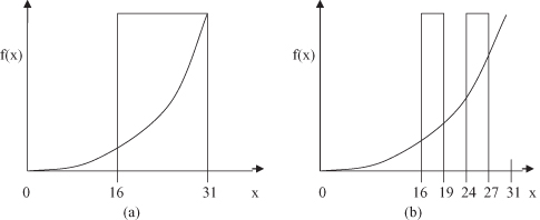
We can graphically illustrate the representation of different schemata for five-bit codes used to optimize the function f(x) = x
2
on interval [0, 31]. Every schema represents a subspace in the 2-D space of the problem. For example, the schema 1**** reduces the search space of the solutions on the subspace given in Figure
13.5
a, and the schema 1*0** has a corresponding search space in Figure
13.5
b.
Figure 13.5.
f(x) = x
2
: Search spaces for different schemata. (a) Schema 1****; (b) Schema 1*0**.
Different schemata have different characteristics. There are three important schema properties:
order
(O),
length
(L), and
fitness
(F). The
order
of the schema S denoted by O(S) is the number of 0 and 1 positions, that is, fixed positions presented in the schema. A computation of the parameter is very simple: It is the length of the template minus the number of
don’t care
symbols. For example, the following three schemata, each of length 10


have the following orders:

The schema S
3
is the most specific one and the schema S
2
is the most general one. The notation of the order of a schema is useful in calculating survival probabilities of the schema for mutations.
The
length
of the schema S, denoted by L(S), is the distance between the first and the last fixed-string positions. It defines the compactness of information contained in a schema. For example, the values of this parameter for the given schemata S
1
to S
3
are

Note that the schema with a single fixed position has a length of 0. The length L of a schema is a useful parameter in calculating the survival probabilities of the schema for crossover.
Another property of a schema S is its
fitness
F(S, t) at time t (i.e., for the given population). It is defined as the average fitness of all strings in the population matched by the schema S. Assume there are p strings {v
1
, v
2
, … , v
p
} in a population matched by a schema S at the time t. Then

The fundamental theorem of schema construction given in this book without proof explains that the
short
(high O),
low-order
(low L), and
above-average
schemata (high F) receive an exponentially increasing number of strings in the next generations of a GA. An immediate result of this theorem is that GAs explore the search space by short, low-order schemata that subsequently are used for information exchange during crossover and mutation operations. Therefore, a GA seeks near-optimal performance through the analysis of these schemata, called the
building blocks
. Note, however, that the building-blocks approach is just a question of empirical results without any proof, and these rules for some real-world problems are easily violated.
13.5 TSP
In this section, we explain how a GA can be used to approach the TSP. Simply stated, the traveling salesman must visit every city in his territory exactly once and then return to the starting point. Given the cost of travel between all the cities, how should he plan his itinerary at a minimum total cost for the entire tour? The TSP is a problem in combinatorial optimization and arises in numerous applications. There are several branch-and-bound algorithms, approximate algorithms, and heuristic search algorithms that approach this problem. In the last few years, there have been several attempts to approximate the TSP solution using GA.
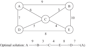
The TSP description is based on a graph representation of data. The problem could be formalized as: Given an undirected weighted graph, find the shortest route, that is, a shortest path in which every vertex is visited exactly once, except that the initial and terminal vertices are the same. Figure
13.6
shows an example of such a graph and its optimal solution. A, B, C, and so on, are the cities that were visited, and the numbers associated with the edges are the cost of travel between the cities.
Figure 13.6.
Graphical representation of the traveling-salesman problem with a corresponding optimal solution.
It is natural to represent each solution of the problem, even if it is not optimal, as a permutation of the cities. The terminal city can be omitted in the representation since it should always be the same as the initial city. For the computation of the total distance of each tour, the terminal city must be counted.
By representing each solution as a permutation of the cities, each city will be visited exactly once. Not every permutation, however, represents a valid solution, since some cities are not directly connected (e.g., A and E in Fig. 10.6). One practical approach is to assign an artificially large distance between cities that are not directly connected. In this way, invalid solutions that contain consecutive, nonadjacent cities will disappear, and all solutions will be allowed.
Our objective here is to minimize the total distance of each tour. We can select different fitness functions that will reflect this objective. For example, if the total distance is s, then f(s) could be a simple f(s) = s if we minimize the fitness function; alternatives for the maximization of a fitness function are f(s) = 1/s, f(s) = 1/s
2
, f(s) = K − s, where K is a positive constant that makes f(s) ≥ 0. There is no general formula to design the best fitness function. But, when we do not adequately reflect the goodness of the solution in the fitness function, finding an optimal or near-optimal solution will not be effective.
When dealing with permutations as solutions, simple crossover operations will result in invalid solutions. For example, for the problem in Figure 10.6, a crossover of two solutions after the third position in the strings
