Data Mining (134 page)
Authors: Mehmed Kantardzic
The Survey Plot is a simple technique of extending an n-dimensional point (sample) in a line graph. Each dimension of the sample is represented on a separate axis in which the dimension’s value is a proportional line from the center of the axis. The principles of representation are given in Figure
15.1
.
Figure 15.1.
A 4-dimensional survey plot.

This visualization of n-dimensional data allows you to see correlations between any two variables, especially when the data are sorted according to a particular dimension. When color is used for different classes of samples, you can sometimes use a sort to see which dimensions are best at classifying data samples. This technique was evaluated with different machine-learning data sets and it showed the ability to present exact IF-THEN rules in a set of samples.
The
Andrews’s curves
technique plots each n-dimensional sample as a curved line. This is an approach similar to a Fourier transformation of a data point. This technique uses the function f(t) in the time domain t to transform the n-dimensional point X = (x1, x2, x3, … , xn) into a continuous plot. The function is usually plotted in the interval −π ≤ t ≤ π. An example of the transforming function f(t) is

One advantage of this visualization is that it can represent many dimensions; the disadvantage, however, is the computational time required to display each n-dimensional point for large data sets.
The class of geometric-projection techniques also includes techniques of exploratory statistics such as principal component analysis (PCA), factor analysis, and multidimensional scaling. Parallel coordinate–visualization technique and radial-visualization technique belong in this category of visualizations, and they are explained in the next sections.
Another class of techniques for visual data mining is the
icon-based techniques
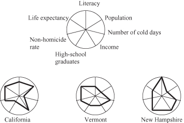
or iconic-display techniques. The idea is to map each multidimensional data item to an icon. An example is the stick-figure technique. It maps two dimensions to the display dimensions and the remaining dimensions are mapped to the angles and/or limb lengths of the stick-figure icon. This technique limits the number of dimensions that can be visualized. A variety of special symbols have been invented to convey simultaneously the variations on several dimensions for the same sample. In 2-D displays, these include Chernoff’s faces, glyphs, stars, and color mapping. Glyphs represent samples as complex symbols whose features are functions of data. We think of glyphs as location-independent representations of samples. For a successful use of glyphs, however, some sort of suggestive layout is often essential, because comparison of glyph shapes is what this type of rendering primarily does. If glyphs are used to enhance a scatter plot, the scatter plot takes over the layout functions. Figure
15.2
shows how the other icon-based technique, called a
star display,
is applied to quality of life measures for various states. Seven dimensions represent seven equidistant radiuses for a circle: one circle for each sample. Every dimension is normalized on interval [0, 1], where the value 0 is in the center of the circle and the value 1 is at the end of the corresponding radius. This representation is convenient for a relatively large number of dimensions but for a very small number of samples. It is usually used for comparative analyses of samples, and it may be included as a part of more complex visualizations.
Figure 15.2.
A star display for data on seven quality-of-life measures for three states.
The other approach is an icon-based, shape-coding technique that visualizes an arbitrary number of dimensions. The icon used in this approach maps each dimension to a small array of pixels and arranges the pixel arrays of each data item into a square or a rectangle. The pixels corresponding to each of the dimensions are mapped to a gray scale or color according to the dimension’s data value. The small squares or rectangles corresponding to the data items or samples are then arranged successively in a line-by-line fashion.
The third class of visualization techniques for multidimensional data aims to map each data value to a colored pixel and present the data values belonging to each attribute in separate windows. Since the
pixel-oriented techniques
use only one pixel per data value, the techniques allow a visualization of the largest amount of data that are possible on current displays (up to about 1,000,000 data values). If one pixel represents one data value, the main question is how to arrange the pixels on the screen. These techniques use different arrangements for different purposes. Finally, the
hierarchical techniques
of visualization subdivide the k-dimensional space and present the subspaces in a hierarchical fashion. For example, the lowest levels are 2-D subspaces. A common example of hierarchical techniques is dimensional-stacking representation.
Dimensional stacking
is a recursive-visualization technique for displaying high-dimensional data. Each dimension is discretized into a small number of bins, and the display area is broken into a grid of subimages. The number of subimages is based on the number of bins associated with the two “outer” dimensions that are user-specified. The subimages are decomposed further based on the number of bins for two more dimensions. This decomposition process continues recursively until all dimensions have been assigned.
Some of the novel visual metaphors that combine data-visualization techniques are already built into advanced visualization tools, and they include:
1.
Parabox.
It combines boxes, parallel coordinates, and bubble plots for visualizing n-dimensional data. It handles both continuous and categorical data. The reason for combining box and parallel-coordinate plots involves their relative strengths. Box plots work well for showing distribution summaries. The strength of parallel coordinates is their ability to display high-dimensional outliers, individual cases with exceptional values. Details about this class of visualization techniques are given in Section 15.3.
2.
Data Constellations.
A component for visualizing large graphs with thousands of nodes and links. Two tables parametrize Data Constellations, one corresponding to nodes and another to links. Different layout algorithms dynamically position the nodes so that patterns emerge (a visual interpretation of outliers, clusters, etc.).
3.
Data Sheet.
A dynamic scrollable text visualization that bridges the gap between text and graphics. The user can adjust the zoom factor, progressively displaying smaller and smaller fonts, eventually switching to a one-pixel representation. This process is called smashing.
4.
Time Table.
a technique for showing thousands of time-stamped events.
5.
Multiscape.
A landscape visualization that encodes information using 3-D “skyscrapers” on a 2-D landscape.
An example of one of these novel visual representations is given in Figure
15.3
, where a large graph is visualized using the Data Constellations technique with one possible graph-layout algorithm.
Figure 15.3.
Data Constellations as a novel visual metaphor.

For most basic visualization techniques that endeavor to show each item in a data set, such as scatter plots or parallel coordinates, a massive number of items will overload the visualization, resulting in a clutter that both causes scalability problems and hinders the user’s understanding of its structure and contents. New visualization techniques have been proposed to overcome data overload problem, and to introduce abstractions that reduce the amount of items to display either in data space or in visual space. The approach is based on coupling aggregation in data space with a corresponding visual representation of the aggregation as a visual entity in the graphical space. This visual aggregate can convey additional information about the underlying contents, such as an average value, minima and maxima, or even its data distribution.
Drawing visual representations of abstractions performed in data space allows for creating simplified versions of visualization while still retaining the general overview. By dynamically changing the abstraction parameters, the user can also retrieve details-on-demand. There are several algorithms to perform data aggregations in a visualization process. For example, given a set of data items,
hierarchical aggregation
is based on iteratively building a tree of aggregates either bottom-up or top-down. Each aggregate item consists of one or more children that are either the original data items (leaves) or aggregate items (nodes). The root of the tree is an aggregate item that represents the entire data set. One of the main visual aggregations for scatter plots involves hierarchical aggregations of data into hulls, as it is represented in Figure
15.4
. Hulls are variations and extensions of rectangular boxes as aggregates. They show enhanced displayed dimensions by using 2-D or 3-D convex hulls instead of axis-aligned boxes as a constrained visual metric. Clearly, the benefit of a data aggregate hierarchy and corresponding visual aggregates is that the resulting visualization can be adapted to the requirements of the human user as well as the technical limitations of the visualization platform.
Figure 15.4.
Convex hull aggregation [Elmquist 2010].
