Data Mining (65 page)

Competitive (or winner-take-all) neural networks are often used to cluster input data where the number of output clusters is given in advance. Well-known examples of ANNs used for clustering based on unsupervised inductive learning include Kohonen’s learning vector quantization (LVQ), self-organizing map (SOM), and networks based on adaptive-resonance theory models. Since the competitive network discussed in this chapter is very closely related to the Hamming networks, it is worth reviewing the key concepts associated with this general and very important class of ANNs. The Hamming network consists of two layers. The first layer is a standard, feedforward layer, and it performs a correlation between the input vector and the preprocessed output vector. The second layer performs a competition to determine which of the preprocessed output vectors is closest to the input vector. The index of the second-layer neuron with a stable, positive output (the winner of the competition) is the index of the prototype vector that best matches the input.

Competitive learning makes efficient adaptive classification, but it suffers from a few methodological problems. The first problem is that the choice of learning rate η forces a trade-off between speed of learning and the stability of the final weight factors. A learning rate near 0 results in slow learning. Once a weight vector reaches the center of a cluster, however, it will tend to stay close to the center. In contrast, a learning rate near 1 results in fast but unstable learning. A more serious stability problem occurs when clusters are close together, which causes weight vectors also to become close, and the learning process switches its values and corresponding classes with each new example. Problems with the stability of competitive learning may occur also when a neuron’s initial weight vector is located so far from any input vector that it never wins the competition, and therefore it never learns. Finally, a competitive-learning process always has as many clusters as it has output neurons. This may not be acceptable for some applications, especially when the number of clusters is not known or if it is difficult to estimate it in advance.

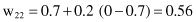
The following example will trace the steps in the computation and learning process of competitive networks. Suppose that there is a competitive network with three inputs and three outputs. The task is to group a set of 3-D input samples into three clusters. The network is fully connected; there are connections between all inputs and outputs and there are also lateral connections between output nodes. Only local feedback weights are equal to 0, and these connections are not represented in the final architecture of the network. Output nodes are based on a linear-activation function with the bias value for all nodes equal to zero. The weight factors for all connections are given in Figure
7.14
, and we assume that the network is already trained with some previous samples.

Figure 7.14.
Example of a competitive neural network.

Suppose that the new sample vector X has components

In the first, forward phase, the temporary outputs for competition are computed through their excitatory connections and their values are

and after including lateral inhibitory connections:

Competition between outputs shows that the highest output value is net
₂
, and it is the winner. So the final outputs from the network for a given sample will be

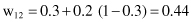
Based on the same sample, in the second phase of competitive learning, the procedure for a weight factor’s correction (only for the winning node y
₂
) starts. The results of the adaptation of the network, based on learning rate η = 0.2, are new weight factors: