Data Mining (66 page)
Authors: Mehmed Kantardzic
The other weight factors in the network remain unchanged because their output nodes were not the winners in the competition for this sample. New weights are the results of a competitive-learning process only for one sample. The process repeats iteratively for large training data sets.
7.7 SOMs
SOMs, often called Kohonen maps, are a data visualization technique introduced by University of Helsinki Professor Teuvo Kohonen,. The main idea of the SOMs is to project the n-dimensional input data into some representation that could be better understood visually, for example, in a 2-D image map. The SOM algorithm is not only a heuristic model used to visualize, but also to explore linear and nonlinear relationships in high-dimensional data sets. SOMs were first used in the 1980s for speech-recognition problems, but later they become a very popular and often used methodology for a variety of clustering and classification-based applications.
The problem that data visualization attempts to solve is: Humans simply cannot visualize high-dimensional data, and SOM techniques are created to help us visualize and understand the characteristics of these dimensional data. The SOM’s output emphasizes on the salient features of the data, and subsequently leads to the automatic formation of clusters of similar data items. SOMs are interpreted as unsupervised neural networks (without teacher) and they are solving clustering problem by visualization of clusters. As a result of a learning process, SOM is used as an important visualization and data-reduction aid as it gives a complete picture of the data; similar data items are transformed in lower dimension but still automatically group together.
The way SOMs perform dimension reduction is by producing an output map of usually one or two dimensions that plot the similarities of the data by grouping similar data items on the map. Through these transformations SOMs accomplish two goals: They reduce dimensions and display similarities. Topological relationships in input samples are preserved while complex multidimensional data can be represented in a lower dimensional space.
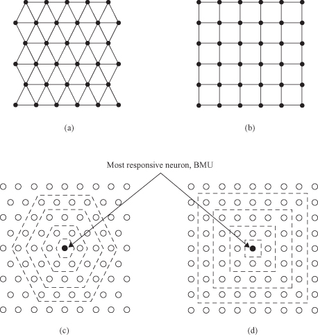
The basic SOM can be visualized as a neural network whose nodes become specifically tuned to various input sample patterns or classes of patterns in an orderly fashion. Nodes with weighted connections are sometimes referred to as neurons since SOMs are actually a specific type of ANNs. SOM is represented as a single layer feedforward network where the output neurons are arranged usually in a 2-D topological grid. The output grid can be either rectangular or hexagonal. In the first case each neuron except borders and corners has four nearest neighbors, in the second there are six. The hexagonal map requires more calculations, but final visualization provides a smoother result. Attached to every output neuron there is a weight vector with the same dimensionality as the input space. Each node
i
has a corresponding weight vector w
i
= {w
i1
,w
i2
, … , w
id
} where d is a dimension of the input feature space.
The structure of the SOM outputs may be a 1-D array or a 2-D matrix, but may also be more complex structures in 3-D such as cylinder or toroid. Figure
7.15
shows an example of a simple SOM architecture with all interconnections between inputs and outputs.
Figure 7.15.
SOM with 2-D Input, 3 × 3 Output.
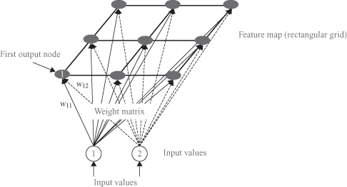
An important part of an SOM technique is the data. These are the samples used for SOM learning. The learning process is competitive and unsupervised, meaning that no teacher is needed to define the correct output for a given input. Competitive learning is used for training the SOM, that is, output neurons compete among themselves to share the input data samples. The winning neuron, with weights w
w
, is a neuron that is the “closest” to the input example x among all other m neurons in the defined metric:
In the basic version of SOMs, only one output node (winner) at a time is activated corresponding to each input. The winner-take-all approach reduces the distance between winner’s node weight vector and the current input sample, making the node closer to be “representative” for the sample. The SOM learning procedure is an iterative process that finds the parameters of the network (weights w) in order to organize the data into clusters that keep the topological structure. Thus, the algorithm finds an appropriate projection of high-dimensional data into a low-dimensional space.
The first step of the SOM learning is the initialization of the neurons’ weights where two methods are widely used. Initial weights can be taken as the coordinates of randomly selected m points from the data set (usually normalized between 0 and 1), or small random values can be sampled evenly from the input data subspace spanned by the two largest principal component eigenvectors. The second method can increase the speed of training but may lead to a local minima and miss some nonlinear structures in the data.
The learning process is performed after initialization where training data set is submitted to the SOM one by one, sequentially, and usually in several iterations. Each output with its connections, often called a cell, is a node containing a template against which input samples are matched. All output nodes are compared with the same input sample in parallel, and SOM computes the distances between each cell and the input. All cells compete, so that only the cell with the closest match between the input and its template produces an active output. Each node therefore acts like a separate decoder or pattern detector for the same input sample, and the winning node is commonly known as the Best Matching Unit (BMU).
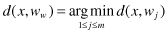
When the winning node is determined for a given input sample, the learning phase adapts the weight vectors in the SOM. Adaptation of the weight vectors for each output occurs through a process similar to competitive learning except that subsets of nodes are adapted at each learning step in order to produce topologically ordered maps. The “winning” node BMU aligns its own weight vector with the training input and hence becomes sensitive to it and will provide maximum response if it is shown to the network again after training. Nodes in the neighborhood set of the “winning” node must also be modified in a similar way to create regions of nodes that will respond to related samples. Nodes outside the neighborhood set remain unchanged. Figure
7.16
a gives an example of 2-D matrix outputs for SOM. For the given BMU the neighborhood is defined as a 3 × 3 matrix of nodes surrounding BMU.
Figure 7.16.
Characteristics of SOM learning process. (a) SOM: BMU and neighborhood; (b) the radius of the neighborhood diminishes with each sample and iteration; (c) BEFORE learning, rectangular grid of SOM; (d) AFTER learning, rectangular grid of SOM.
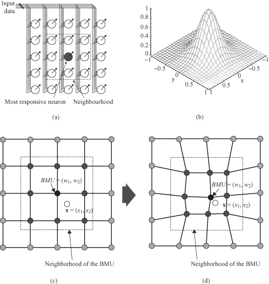
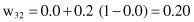
Every node within the BMU’s neighborhood (including the BMU) has its weight vector adjusted according to the following equation in the iterative training process:

where
h
i
(
t
) is a so-called neighborhood function. It is defined as a function of time t or more precisely a training iteration, and it specifies the neighborhood area of the
i
th neuron. It has been found experimentally that in order to achieve global ordering of the map the neighborhood set around the winning node should initially be large to quickly produce a rough mapping. With the increased number of iterations through the training set data, the neighborhood should be reduced to force a more localized adaptation of the network. This is done so the input samples can first move to an area of SOM where they will probably be, and then they will more precisely determine the position. This process is similar to coarse adjustment followed by fine-tuning (Fig.
7.17
). The radius of the neighborhood of the BMU is therefore dynamic. To do this SOM can use, for example, the
exponential decay function
that reduces the radius dynamically with each new iteration. The graphical interpretation of the function is given in Figure
7.16
b.
Figure 7.17.
Coarse adjustment followed by fine-tuning through the neighborhood. (a) Hexagonal grid; (b) rectangular grid; (c) neighborhood in a hexagonal grid; (d) neighborhood in a rectangular grid.