Data Mining (68 page)

15.
Is it true that the Vapnik-Chervonenkis (VC) dimension of a perceptron is smaller than the VC dimension of a simple linear support vector machine (SVM)? Discuss your answer.

7.9 REFERENCES FOR FURTHER STUDY

Engel, A., C. Van den Broeck,
Statistical Mechanics of Learning
, Cambridge University Press, Cambridge, UK, 2001.

The subject of this book is the contribution made to machine learning over the last decade by researchers applying the techniques of statistical mechanics. The authors provide a coherent account of various important concepts and techniques that are currently only found scattered in papers. They include many examples and exercises to make a book that can be used with courses, or for self-teaching, or as a handy reference.

Haykin, S.,
Neural Networks and Learning Machines
, 3rd edition, Prentice Hall, Upper Saddle River, NJ, 2009.

Fluid and authoritative, this well-organized book represents the first comprehensive treatment of neural networks from an engineering perspective, providing extensive, state-of-the-art coverage that will expose readers to the myriad facets of neural networks and help them appreciate the technology’s origin, capabilities, and potential applications. The book examines all the important aspects of this emerging technology, covering the learning process, backpropagation, radial basis functions, recurrent networks, self-organizing systems, modular networks, temporal processing, neurodynamics, and VLSI implementation. It integrates computer experiments throughout to demonstrate how neural networks are designed and perform in practice. Chapter objectives, problems, worked examples, a bibliography, photographs, illustrations, and a thorough glossary all reinforce concepts throughout. New chapters delve into such areas as SVMs, and reinforcement learning/neurodynamic programming, plus readers will find an entire chapter of case studies to illustrate the real-life, practical applications of neural networks. A highly detailed bibliography is included for easy reference. It is the book for professional engineers and research scientists.

Heaton, J.,
Introduction to Neural Networks with Java
, Heaton Research, St. Louis, MO, 2005.

Introduction to
Neural Networks with Java
introduces the Java programmer to the world of neural networks and artificial intelligence (AI). Neural-network architectures such as the feedforward backpropagation, Hopfield, and Kohonen networks are discussed. Additional AI topics, such as Genetic Algorithms and Simulated Annealing, are also introduced. Practical examples are given for each neural network. Examples include the Traveling Salesman problem, handwriting recognition, fuzzy logic, and learning mathematical functions. All Java source code can be downloaded online. In addition to showing the programmer how to construct these neural networks, the book discusses the Java Object Oriented Neural Engine (JOONE). JOONE is a free open source Java neural engine.

Principe, J. C., R. Mikkulainen,
Advances in Self-Organizing Maps, Series: Lecture Notes in Computer Science
, Vol. 5629, Springer, New York, 2009.

This book constitutes the refereed proceedings of the 7th International Workshop on Advances in Self-Organizing Maps, WSOM 2009, held in St. Augustine, Florida, in June 2009. The 41 revised full papers presented were carefully reviewed and selected from numerous submissions. The papers deal with topics in the use of SOM in many areas of social sciences, economics, computational biology, engineering, time-series analysis, data visualization, and theoretical computer science.

Zurada, J. M.,
Introduction to Artificial Neural Systems
, West Publishing Co., St. Paul, MN, 1992.

The book is one of the traditional textbooks on ANNs. The text grew out of a teaching effort in artificial neural systems offered for both electrical engineering and computer science majors. The author emphasizes that the practical significance of neural computation becomes apparent for large or very large-scale problems.

Chapter Objectives

• Explain the basic characteristics of ensemble learning methodologies.
  
• Distinguish between the different implementations of combination schemes for different learners.
  
• Compare bagging and boosting approaches.
  
• Introduce AdaBoost algorithm and its advantages.
  

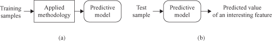
One of the primary goals of data mining is to predict an “unknown” value of a new sample from observed samples. Such a prediction is achieved by two sequential phases as shown in Figure
8.1
: (a) training phase—producing a predictive model from training samples using one of the available supervised learning algorithms; and (b) testing phase—evaluating the generated predictive model using test samples that are not used in the training phase. Numerous applications of a data-mining process showed validity of the so-called “No-Free-Lunch Theorem.” It states that there is no single learning algorithm that is the best and most accurate in all applications. Each algorithm determines a certain model that comes with a set of assumptions. Sometimes these assumptions hold, sometimes not; therefore, no single algorithm “wins” all the time.

Figure 8.1.
Training phase and testing phase for a predictive model. (a) Training phase; (b) testing phase.

In order to improve the accuracy of a predictive model, the promising approach called the
ensemble learning
is introduced. The idea is to combine results from various predictive models generated using training samples. The key motivation behind the proposed approach is to reduce the error rate. An initial assumption is that it will become much more unlikely that the ensemble will misclassify a new sample compared with a single predictive model. When combinining multiple, independent, and diverse “decisions makers,” each of which is at least more accurate than random guessing, correct decisions should be reinforced. The idea may be demonstrated by some simple decision processes where single-human performances are compared with human ensembles. For example, given the question “How many jelly beans are in the jar?”, the group average will outperform individual estimates. Or, in the TV series “Who Wants to be a Millionaire?” where audience (ensemble) vote is a support for the candidate who is not sure of the answer.

This idea is proven theoretically by Hansen and company through the statement: If
N
classifiers make
independent
errors and they have the error probability
e
< 0.5, then it can be shown that the error of an ensemble
E
is monotonically decreasing the function of
N
. Clearly, performances quickly decrease for dependent classifiers.

8.1 ENSEMBLE-LEARNING METHODOLOGIES

The ensemble-learning methodology consists of two sequential phases: (a) the training phase, and (b) the testing phase. In the training phase, the ensemble method generates several different predictive models from training samples as presented in Figure
8.2
a. For predicting an unknown value of a test sample, the ensemble method aggregates outputs of each predictive model (Fig.
8.2
b). An integrated predictive model generated by an ensemble approach consists of several predictive models (Predictive model.1, Predictive model.2, … , Predictive model.
n
) and a combining rule as shown in Figure
8.2
b. We will refer to such a predictive model as an
ensemble
. The field of ensemble learning is still relatively new, and several names are used as synonyms depending on which predictive task is performed, including combination of multiple classifiers, classifier fusion, mixture of experts, or consensus aggregation.

Figure 8.2.
Training phase and testing phase for building an ensemble. (a) Training phase; (b) testing phase.

To perform better than a single predictive model, an ensemble should consist of predictive models that are independent of each other, that is, their errors are uncorrelated, and each of them has an accuracy rate of >0.5. The outcome of each predictive model is aggregated to determine the output value of a test sample. We may analyze all steps of ensemble prediction for a classification task. For example, we may analyze a classification task where the ensemble consists of 15 classifiers, each of which classifies test samples into one of two categorical values. The ensemble decides the categorical value based on the dominant frequency of classifiers’ outputs. If 15 pre­dictive models are different from each other, and each model has the identical error rate (ε = 0.3), the ensemble will make a wrong prediction only if more than half of the predictive models misclassify a test sample. Therefore, the error rate of the ensemble is

which is considerably lower than the 0.3 error rate of a single classifier. The sum is starting with eight, and it means that eight or more models misclassified a test sample, while seven or fewer models classified the sample correctly.

Figure
8.3
a shows the error rates of an ensemble, which consists of 15 predictive models (n = 15). The x-axis represents an error rate (ε) of a single classifier. The diagonal line represents the case in which all models in the ensemble are identical. The solid line represents error rates of an ensemble in which predictive models are different and independent from each other. An ensemble has a significantly lower error rate than a single predictive model only when the error rate (ε) of the members of the ensemble is lower than 0.5.

Figure 8.3.
Changes in error rates of an ensemble. (a) Identical predictive models versus different predictive models in an ensemble; (b) the different number of predictive models in an ensemble.

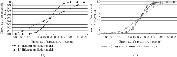
We can also analyze the effect of the number of predictive models in an ensemble. Figure
8.3
b shows error-rate curves for ensembles that consist of 5, 15, 25, and 35 predictive models, respectively. Observe that when an error rate of a predictive model is lower than 0.5, the larger the number of predictive models is, the lower the error rate of an ensemble is. For example, when each predictive model of an ensemble has an error rate of 0.4, error rates of each ensemble (
n
= 5,
n
= 15,
n
= 25, and
n
= 35) are calculated as 0.317, 0.213, 0.153, and 0.114, respectively. However, this decrease in the error rate for an ensemble is becoming less significant if the number of classifiers is very large, or when the error rate of each classifier becomes relatively small.

The basic questions in creating an ensemble learner are as follows: How to generate base learners, and how to combine the outputs from base learners? Diverse and independent learners can be generated by

Stacked Generalization (or stacking) is a methodology that could be classified in the first group (a). Unlike other well-known techniques, stacking may be (and normally is) used to combine models of different types. One way of combining multiple models is specified by introducing the concept of a meta-learner. The learning procedure is as follows:

Note that steps (1) to (3) are the same as cross-validation, but instead of using a winner-take-all approach, the base learners are combined, possibly nonlinearly. Although an attractive idea, it is less theoretically analyzed and less widely used than bagging and boosting, the two most recognized ensemble-learning methodologies. Similar situation is with the second group of methodologies (b): Although a very simple approach, it is not used or analyzed intensively. Maybe the main reason is that applying the same methodology with different parameters does not guarantee independence of models.

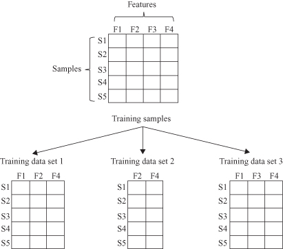
Class (c) methodologies are based on manual or automatic feature selection/extraction that can be used for generating diverse classifiers using different feature sets. For example, subsets related to different sensors, or subsets of features computed with different algorithms, may be used. To form training data sets, different subsets of input features are chosen, and then each training sample with the selected input features becomes an element of training data sets. In Figure
8.4
, there are five training samples {S1, S2, S3, S4, S5} with four features {F1, F2, F3, F4}. When the training data set 1 is generated, three features {F1, F2, F4} is randomly selected from input features {F1, F2, F3, F4}, and all training samples with those features form the first training set. Similar process is performed for the other training sets. The main requirement is that classifiers use different subsets of features that are complementary.

Figure 8.4.
Feature selection for ensemble classifiers methodology.