Data Mining (61 page)
Authors: Mehmed Kantardzic
Figure 7.8.
Block diagram of ANN-based feedback-control system.
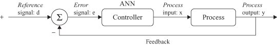
The system involves the use of feedback to control the output y on the level of a reference signal d supplied from the external source. A controller of the system can be realized in an ANN technology. The error signal e, which is the difference between the process output y and the reference value d, is applied to an ANN-based controller for the purpose of adjusting its free parameters. The primary objective of the controller is to supply appropriate inputs x to the process to make its output y track the reference signal d. It can be trained through:
1.
Indirect Learning.
Using actual input–output measurements on the process, an ANN model of a control is first constructed offline. When the training is finished, the ANN controller may be included into the real-time loop.
2.
Direct Learning.
The training phase is online, with real-time data, and the ANN controller is enabled to learn the adjustments to its free parameters directly from the process.
Filtering
The term filter often refers to a device or algorithm used to extract information about a particular quantity from a set of noisy data. Working with series of data in time domain, frequent domain, or other domains, we may use an ANN as a filter to perform three basic information-processing tasks:
1.
Filtering.
This task refers to the extraction of information about a particular quantity at discrete time
n
by using data measured up to and including time
n
.
2.
Smoothing.
This task differs from filtering in that data need not be available only at time
n
; data measured later than time
n
can also be used to obtain the required information. This means that in smoothing there is a delay in producing the result at discrete time
n
.
3.
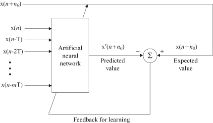
Prediction.
The task of prediction is to forecast data in the future. The aim is to derive information about what the quantity of interest will be like at some time
n
+
n
0
in the future, for
n
0
> 0, by using data measured up to and including time
n
. Prediction may be viewed as a form of model building in the sense that the smaller we make the prediction error, the better the network serves as a model of the underlying physical process responsible for generating the data. The block diagram of an ANN for a prediction task is given in Figure
7.9
.
Figure 7.9.
Block diagram of an ANN-based prediction.
7.5 MULTILAYER PERCEPTRONS (MLPs)
Multilayer feedforward networks are one of the most important and most popular classes of ANNs in real-world applications. Typically, the network consists of a set of inputs that constitute the input layer of the network, one or more hidden layers of computational nodes, and finally an output layer of computational nodes. The processing is in a forward direction on a layer-by-layer basis. This type of ANNs are commonly referred to as MLPs, which represent a generalization of the simple perceptron, a network with a single layer, considered earlier in this chapter.
A multiplayer perceptron has three distinctive characteristics:
1.
The model of each neuron in the network includes usually a nonlinear activation function, sigmoidal or hyperbolic.
2.
The network contains one or more layers of hidden neurons that are not a part of the input or output of the network. These hidden nodes enable the network to learn complex and highly nonlinear tasks by extracting progressively more meaningful features from the input patterns.
3.
The network exhibits a high degree of connectivity from one layer to the next one.
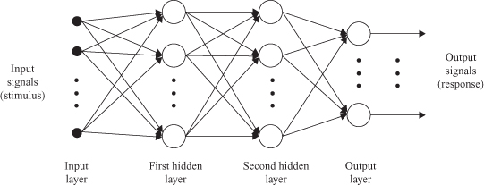
Figure
7.10
shows the architectural graph of a multilayered perceptron with two hidden layers of nodes for processing and an output layer. The network shown here is fully connected. This means that the neuron in any layer of the network is connected to all the nodes (neurons) in the previous layer. Data flow through the network progresses in a forward direction, from left to right and on a layer-by-layer basis.
Figure 7.10.
A graph of a multilayered-perceptron architecture with two hidden layers.
MLPs have been applied successfully to solve some difficult and diverse problems by training the network in a supervised manner with a highly popular algorithm known as the
error backpropagation algorithm
. This algorithm is based on the error-correction learning rule and it may be viewed as its generalization. Basically, error backpropagation learning consists of two phases performed through the different layers of the network: a forward pass and a backward pass.
In the forward pass, a training sample (input data vector) is applied to the input nodes of the network, and its effect propagates through the network layer by layer. Finally, a set of outputs is produced as the actual response of the network. During the forward phase, the synaptic weights of the network are all fixed. During the backward phase, on the other hand, the weights are all adjusted in accordance with an error-correction rule. Specifically, the actual response of the network is subtracted from a desired (target) response, which is a part of the training sample, to produce an error signal. This error signal is then propagated backward through the network, against the direction of synaptic connections. The synaptic weights are adjusted to make the actual response of the network closer to the desired response.
Formalization of the backpropagation algorithm starts with the assumption that an error signal exists at the output of a neuron j at iteration
n
(i.e., presentation of the
n
th training sample). This error is defined by
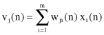
We define the instantaneous value of the error energy for neuron j as 1/2 e
j
2
(
n
). The total error energy for the entire network is obtained by summing instantaneous values over all neurons in the output layer. These are the only “visible” neurons for which the error signal can be calculated directly. We may thus write
where the set C includes all neurons in the output layer of the network. Let N denote the total number of samples contained in the training set. The average squared error energy is obtained by summing E(
n
) over all
n
and then normalizing it with respect to size N, as shown by
The average error energy E
av
is a function of all the free parameters of the network. For a given training set, E
av
represents the cost function as a measure of learning performances. The objective of the learning process is to adjust the free parameters of the network to minimize E
av
. To do this minimization, the weights are updated on a sample-by-sample basis for one iteration, that is, one complete presentation of the entire training set of a network has been dealt with.
To obtain the minimization of the function E
av
, we have to use two additional relations for node-level processing, which have been explained earlier in this chapter: