Data Mining (59 page)

Although many neural-network models have been proposed in both classes, the multilayer feedforward network with a backpropagation-learning mechanism is the most widely used model in terms of practical applications. Probably over 90% of commercial and industrial applications are based on this model. Why multilayered networks? A simple example will show the basic differences in application requirements between single-layer and multilayer networks.

The simplest and well-known classification problem, very often used as an illustration in the neural-network literature, is the exclusive-OR (XOR) problem. The task is to classify a binary input vector X to class 0 if the vector has an even number of 1’s or otherwise assign it to class 1. The XOR problem is not linearly separable; this can easily be observed from the plot in Figure
7.4
for a two-dimensional (2-D) input vector X = {x
₁
, x
₂
}. There is no possibility of obtaining a single linear separation of points that belong to different classes. In other words, we cannot use a single-layer network to construct a straight line (in general, it is a linear hyperplane in an n-dimensional space) to partition the 2-D input space into two regions, each containing data points of only the same class. It is possible to solve the problem with a two-layer network, as illustrated in Figure
7.5
, in which one possible solution for the connection weights and thresholds is indicated. This network generates a nonlinear separation of points in a 2-D space.

Figure 7.4.
XOR problem.

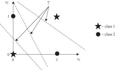
Figure 7.5.
XOR solution: the two-layer ANN with the hard-limit activation function.

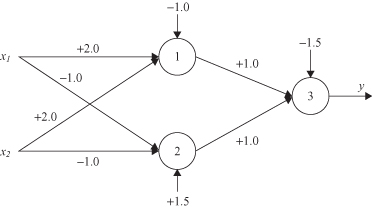
The basic conclusion from this example is that single-layered ANNs are a convenient modeling tool only for relatively simple problems that are based on linear models. For most real-world problems, where models are highly nonlinear, multilayered networks are better and maybe the only solution.

7.3 LEARNING PROCESS

A major task for an ANN is to learn a model of the world (environment) in which it is embedded and to maintain the model sufficiently consistent with the real world so as to achieve the specified goals of the concerned application. The learning process is based on data samples from the real world, and here lies a fundamental difference between the design of an ANN and a classical information-processing system. In the latter case, we usually proceed by first formulating a mathematical model of environmental observations, validating the model with real data, and then building (programming) the system on the basis of the model. In contrast, the design of an ANN is based directly on real-life data, with the data set being permitted to “speak for itself.” Thus, an ANN not only provides the implicit model formed through the learning process, but also performs the information-processing function of interest.

The property that is of primary significance for an ANN is the ability of the network to learn from its environment based on real-life examples, and to improve its performance through that learning process. An ANN learns about its environment through an interactive process of adjustments applied to its connection weights. Ideally, the network becomes more knowledgeable about its environment after each iteration in the learning process. It is very difficult to agree on a precise definition of the term learning. In the context of ANNs one possible definition of inductive learning is as follows:

Learning is a process by which the free parameters of a neural network are adapted through a process of stimulation by the environment in which the network is embedded. The type of learning is determined by the manner in which the parameters change.

A prescribed set of well-defined rules for the solution of a learning problem is called a learning algorithm. Basically, learning algorithms differ from each other in the way in which the adjustment of the weights is formulated. Another factor to be considered in the learning process is the manner in which ANN architecture (nodes and connections) is built.

To illustrate one of the learning rules, consider the simple case of a neuron k, shown in Figure
7.1
, constituting the only computational node of the network. Neuron
k
is driven by input vector X(
n
), where
n
denotes discrete time, or, more precisely, the time step of the iterative process involved in adjusting the input weights w
_ki
. Every data sample for ANN training (learning) consists of the input vector X(
n
) and the corresponding output d(
n
).

Processing the input vector X(
n
), a neuron k produces the output that is denoted by y
_k
(
n
):

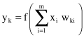
It represents the only output of this simple network, and it is compared with a desired response or target output d
_k
(
n
) given in the sample. An error e
_k
(
n
) produced at the output is by definition

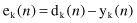
The error signal produced actuates a control mechanism of the learning algorithm, the purpose of which is to apply a sequence of corrective adjustments to the input weights of a neuron. The corrective adjustments are designed to make the output signal y
_k
(
n
) come closer to the desired response d
_k
(
n
) in a step-by-step manner. This objective is achieved by minimizing a cost function E(
n
), which is the instantaneous value of error energy, defined for this simple example in terms of the error e
_k
(
n
):

The learning process based on a minimization of the cost function is referred to as
error-correction learning
. In particular, minimization of E(
n
) leads to a learning rule commonly referred to as the
delta rule
or Widrow-Hoff rule. Let w
_kj
(
n
) denote the value of the weight factor for neuron
k
excited by input x
_j
(
n
) at time step
n
. According to the delta rule, the adjustment Δw
_kj
(
n
) is defined by

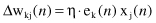
where η is a positive constant that determines the rate of learning. Therefore, the delta rule may be stated as: The adjustment made to a weight factor of an input neuron connection is proportional to the product of the error signal and the input value of the connection in question.

Having computed the adjustment Δw
_kj
(
n
), the updated value of synaptic weight is determined by

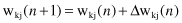
In effect, w
_kj
(
n
) and w
_kj
(
n
+ 1) may be viewed as the old and new values of synaptic weight w
_kj
, respectively. From Figure
7.6
we recognize that error-correction learning is an example of a closed-loop feedback system. Control theory explains that the stability of such a system is determined by those parameters that constitute the feedback loop. One of those parameters of particular interest is the learning rate η. This parameter has to be carefully selected to ensure that the stability of convergence of the iterative-learning process is achieved. Therefore, in practice, this parameter plays a key role in determining the performance of error-correction learning.