Data Mining (57 page)
Authors: Mehmed Kantardzic
Find the best threshold (for the maximal gain) for AttributeA.
(a)
Find the best threshold (for the maximal gain) for AttributeB.
(b)
Find a decision tree for data set Y.
(c)
If the testing set is: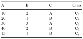
What is the percentage of correct classifications using the decision tree developed in (c).
(d)
Derive decision rules from the decision tree.
5.
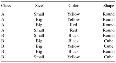
Use the C4.5 algorithm to build a decision tree for classifying the following objects:
6.
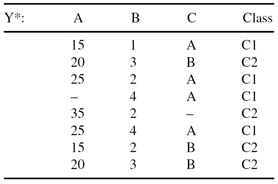
Given a training data set Y* with missing values:
(a)
Apply a modified C4.5 algorithm to construct a decision tree with the (T
i
/E) parameters explained in Section 7.3.
(b)
Analyze the possibility of pruning the decision tree obtained in (a).
(c)
Generate decision rules for the solution in (a). Is it necessary to generate a default rule for this rule-based model?
7.
Why is postpruning in C4.5 defined as pessimistic pruning?
8.
Suppose that two decision rules are generated with C4.5:
| Rule1: | (X > 3) ∧ (Y ≥ 2) → Class1 (9.6/0.4) |
| Rule2: | (X > 3) ∧ (Y < 2) → Class2 (2.4/2.0). |
Analyze if it is possible to generalize these rules into one using confidence limit U
25%
for the binomial distribution.
9.
Discuss the complexity of the algorithm for optimal splitting of numeric attributes into more than two intervals.
10.
In real-world data-mining applications, a final model consists of extremely large number of decision rules. Discuss the potential actions and analyses you should perform to reduce the complexity of the model.
11.
Search the Web to find the basic characteristics of publicly available or commercial software tools for generating decision rules and decision trees. Document the results of your search.
12.
Consider a binary classification problem (output attribute value = {Low, High}) with the following set of input attributes and attribute values:
- Air Conditioner = {Working, Broken}
- Engine = {Good, Bad}
- Mileage = {High, Medium, Low}
- Rust = {Yes, No}
Suppose a rule-based classifier produces the following rule set:
Mileage
=
High
−→
Value
=
Low
Mileage
=
Low
−→
Value
=
High
Air Conditioner
=
Working and Engine
=
Good
−→
Value
=
High
Air Conditioner
=
Working and Engine
=
Bad
−→
Value
=
Low
Air Conditioner
=
Broken
−→
Value
=
Low
(a)
Are the rules mutually exclusive? Explain your answer.
(b)
Is the rule set exhaustive (covering each possible case)? Explain your answer.
(c)
Is ordering needed for this set of rules? Explain your answer.
(d)
Do you need a default class for the rule set? Explain your answer.
13.
Of the following algorithms:
- C4.5
- K-Nearest Neighbor
- Naïve Bayes
- Linear Regression
(a)
Which are fast in training but slow in classification?(b)
Which one produces classification rules?(c)
Which one requires discretization of continuous attributes before application?(d)
Which model is the most complex?
14.
(a)
How much information is involved in choosing one of eight items, assuming that they have an equal frequency?
(b)
One of 16 items?
15.
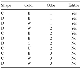
The following data set will be used to learn a decision tree for predicting whether a mushroom is edible or not based on its shape, color, and odor.
(a)
What is entropy H(Edible|Odor = 1 or Odor = 3)?
(b)
Which attribute would the C4.5 algorithm choose to use for the root of the tree?
(c)
Draw the full decision tree that would be learned for this data (no pruning).
(d)
Suppose we have a validation set as follows. What will be the training set error and validation set error of the tree? Express your answer as the number of examples that would be misclassified.
6.9 REFERENCES FOR FURTHER STUDY
Dzeroski, S., N. Lavrac, eds.,
Relational Data Mining
, Springer-Verlag, Berlin, Germany, 2001.
Relational data mining has its roots in inductive logic programming, an area in the intersection of machine learning and programming languages. The book provides a thorough overview of different techniques and strategies used in knowledge discovery from multi-relational data. The chapters describe a broad selection of practical, inductive-logic programming approaches to relational data mining, and give a good overview of several interesting applications.
Kralj Novak, P., N. Lavrac, G. L. Webb, Supervised Descriptive Rule Discovery: A Unifying Survey of Contrast Set, Emerging Pattern and Subgroup Mining,
Journal of Machine Learning Research
, Vol. 10, 2009, p. 377–403.
This paper gives a survey of contrast set mining (CSM), emerging pattern mining (EPM), and subgroup discovery (SD) in a unifying framework named
supervised descriptive rule discovery
. While all these research areas aim at discovering patterns in the form of rules induced from labeled data, they use different terminology and task definitions, claim to have different goals, claim to use different rule learning heuristics, and use different means for selecting subsets of induced patterns. This paper contributes a novel understanding of these subareas of data mining by presenting a unified terminology, by explaining the apparent differences between the learning tasks as variants of a unique supervised descriptive rule discovery task and by exploring the apparent differences between the approaches.
Mitchell, T.,
Machine Learning
, McGraw Hill, New York, NY, 1997.
This is one of the most comprehensive books on machine learning. Systematic explanations of all methods and a large number of examples for all topics are the main strengths of the book. Inductive machine-learning techniques are only a part of the book, but for a deeper understanding of current data-mining technology and newly developed techniques, it is very useful to get a global overview of all approaches in machine learning.
Quinlan, J. R.,
C4.5: Programs for Machine Learning
, Morgan Kaufmann, San Mateo, CA, 1992.
The book outlines the C4.5 algorithm step by step, with detailed explanations and many illustrative examples. The second part of the book is taken up by the source listing of the C program that makes up the C4.5 system. The explanations in the book are intended to give a broad-brush view of C4.5 inductive learning with many small heuristics, leaving the detailed discussion to the code itself.
Russell, S., P. Norvig,
Artificial Intelligence: A Modern Approach
, Prentice Hall, Upper Saddle River, NJ, 1995.
The book gives a unified presentation of the artificial intelligence field using an agent-based approach. Equal emphasis is given to theory and practice. An understanding of the basic concepts in artificial intelligence (AI), including an approach to inductive machine learning, is obtained through layered explanations and agent-based implementations of algorithms.
7
ARTIFICIAL NEURAL NETWORKS
Chapter Objectives
- Identify the basic components of artificial neural networks (ANNs) and their properties and capabilities.
- Describe common learning tasks such as pattern association, pattern recognition, approximation, control, and filtering that are performed by ANNs.
- Compare different ANN architecture such as feedforward and recurrent networks, and discuss their applications.
- Explain the learning process at the level of an artificial neuron, and its extension for multiplayer, feedforward-neural networks.
- Compare the learning processes and the learning tasks of competitive networks and feedforward networks.
- Present the basic principles of Kohonen maps and their applications.
- Discuss the requirements for good generalizations with ANNs based on heuristic parameter tuning.
Work on ANNs has been motivated by the recognition that the human brain computes in an entirely different way from the conventional digital computer. It was a great challenge for many researchers in different disciplines to model the brain’s computational processes. The brain is a highly complex, nonlinear, and parallel information-processing system. It has the capability to organize its components and to perform certain computations with a higher quality and many times faster than the fastest computer in existence today. Examples of these processes are pattern recognition, perception, and motor control. ANNs have been studied for more than four decades since Rosenblatt first applied the
single-layer perceptrons
to pattern-classification learning in the late 1950s.
An ANN is an abstract computational model of the human brain. The human brain has an estimated 10
11
tiny units called neurons. These neurons are interconnected with an estimated 10
15
links. Similar to the brain, an ANN is composed of artificial neurons (or processing units) and interconnections. When we view such a network as a graph, neurons can be represented as nodes (or vertices) and interconnections as edges. Although the term ANN is most commonly used, other names include “neural network,” parallel distributed processing (PDP) system, connectionist model, and distributed adaptive system. ANNs are also referred to in the literature as neurocomputers.
A neural network, as the name indicates, is a network structure consisting of a number of nodes connected through directional links. Each node represents a processing unit, and the links between nodes specify the causal relationship between connected nodes. All nodes are adaptive, which means that the outputs of these nodes depend on modifiable parameters pertaining to these nodes. Although there are several definitions and several approaches to the ANN concept, we may accept the following definition, which views the ANN as a formalized adaptive machine:
An ANN is a massive parallel distributed processor made up of simple processing units. It has the ability to learn experiential knowledge expressed through interunit connection strengths, and can make such knowledge available for use.
It is apparent that an ANN derives its computing power through, first, its massive parallel distributed structure and, second, its ability to learn and therefore to generalize. Generalization refers to the ANN producing reasonable outputs for new inputs not encountered during a learning process. The use of ANNs offers several useful properties and capabilities:
1.
Nonlinearity.
An artificial neuron as a basic unit can be a linear-or nonlinear-processing element, but the entire ANN is highly nonlinear. It is a special kind of nonlinearity in the sense that it is distributed throughout the network. This characteristic is especially important, for ANN models the inherently nonlinear real-world mechanisms responsible for generating data for learning.
2.
Learning from Examples.
An ANN modifies its interconnection weights by applying a set of training or learning samples. The final effects of a learning process are tuned parameters of a network (the parameters are distributed through the main components of the established model), and they represent implicitly stored knowledge for the problem at hand.
3.
Adaptivity.
An ANN has a built-in capability to adapt its interconnection weights to changes in the surrounding environment. In particular, an ANN trained to operate in a specific environment can be easily retrained to deal with changes in its environmental conditions. Moreover, when it is operating in a nonstationary environment, an ANN can be designed to adopt its parameters in real time.
4.
Evidential Response.
In the context of data classification, an ANN can be designed to provide information not only about which particular class to select for a given sample, but also about confidence in the decision made. This latter information may be used to reject ambiguous data, should they arise, and thereby improve the classification performance or performances of the other tasks modeled by the network.
5.
Fault Tolerance.
An ANN has the potential to be inherently fault-tolerant, or capable of robust computation. Its performances do not degrade significantly under adverse operating conditions such as disconnection of neurons, and noisy or missing data. There is some empirical evidence for robust computation, but usually it is uncontrolled.
6.
Uniformity of Analysis and Design.
Basically, ANNs enjoy universality as information processors. The same principles, notation, and steps in methodology are used in all domains involving application of ANNs.
To explain a classification of different types of ANNs and their basic principles it is necessary to introduce an elementary component of every ANN. This simple processing unit is called an artificial neuron.
7.1 MODEL OF AN ARTIFICIAL NEURON
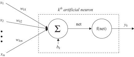
An artificial neuron is an information-processing unit that is fundamental to the operation of an ANN. The block diagram (Fig.
7.1
), which is a model of an artificial neuron, shows that it consists of three basic elements:
1.
A set of connecting links
from different inputs x
i
(or synapses), each of which is characterized by a weight or strength w
ki
. The first index refers to the neuron in question and the second index refers to the input of the synapse to which the weight refers. In general, the weights of an artificial neuron may lie in a range that includes negative as well as positive values.
2.
An adder
for summing the input signals x
i
weighted by the respective synaptic strengths w
ki
. The operation described here constitutes a linear combiner.
3.
An activation function
f for limiting the amplitude of the output y
k
of a neuron.
Figure 7.1.
Model of an artificial neuron.
The model of the neuron given in Figure
7.1
also includes an externally applied bias, denoted by b
k
. The bias has the effect of increasing or lowering the net input of the activation function, depending on whether it is positive or negative.
In mathematical terms, an artificial neuron is an abstract model of a natural neuron, and its processing capabilities are formalized using the following notation. First, there are several inputs x
i
, i = 1, … , m. Each input x
i
is multiplied by the corresponding weight w
ki
where k is the index of a given neuron in an ANN. The weights simulate the biological synaptic strengths in a natural neuron. The weighted sum of products x
i
w
ki
for i = 1, … , m is usually denoted as
net
in the ANN literature:

Using adopted notation for w
k0
= b
k
and default input x
0
= 1, a new uniform version of net summation will be

The same sum can be expressed in vector notation as a scalar product of two m-dimensional vectors:

where
| X | = {x 0 , x 1 , x 2 , … , x m } |
| W | = {w k0 , w k1 , w k2 , … , w km } |
Finally, an artificial neuron computes the output y
k
as a certain function of
net
k
value:

The function f is called the activation function. Various forms of activation functions can be defined. Some commonly used activation functions are given in Table
7.1
.
TABLE 7.1.
A Neuron’s Common Activation Functions
| Activation Function | Input/Output Relation | Graph |
| Hard limit |  | 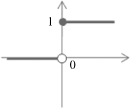 |
| Symmetrical hard limit |  | 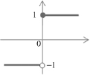 |
| Linear |  | 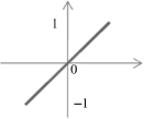 |
| Saturating linear |  | 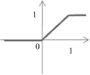 |
| Symmetric saturating linear |  | 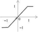 |
| Log-sigmoid |  | 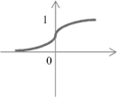 |
| Hyperbolic tangent sigmoid |  | 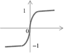 |