Data Mining (54 page)
Authors: Mehmed Kantardzic

Since the existing subtree has a higher value of predicted error than the replaced node, it is recommended that the decision tree be pruned and the subtree replaced with the new leaf node.
6.5 C4.5 ALGORITHM: GENERATING DECISION RULES
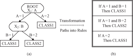
Even though the pruned trees are more compact than the originals, they can still be very complex. Large decision trees are difficult to understand because each node has a specific context established by the outcomes of tests at antecedent nodes. To make a decision-tree model more readable, a path to each leaf can be transformed into an IF-THEN production rule. The IF part consists of all tests on a path, and the THEN part is a final classification. Rules in this form are called
decision rules
, and a collection of decision rules for all leaf nodes would classify samples exactly as the tree does. As a consequence of their tree origin, the IF parts of the rules would be mutually exclusive and exhaustive, so the order of the rules would not matter. An example of the transformation of a decision tree into a set of decision rules is given in Figure
6.10
, where the two given attributes, A and B, may have two possible values, 1 and 2, and the final classification is into one of two classes.
Figure 6.10.
Transformation of a decision tree into decision rules. (a) Decision tree; (b) decision rules.
For our trained decision tree in Figure
6.8
, the corresponding decision rules will be
| If | Attribute1 = A and Attribute2 < = 70 |
| Then Classification = CLASS1 (2.0/0); | |
| If | Attribute1 = A and Attribute2 > 70 |
| Then Classification = CLASS2 (3.4/0.4); | |
| If | Attribute1 = B |
| Then Classification = CLASS1 (3.2/0); | |
| If | Attribute1 = C and Attribute3 = True |
| Then Classification = CLASS2 (2.4/0); | |
| If | Attribute1 = C and Attribute3 = False |
| Then Classification = CLASS1 (3.0/0). |
Rewriting the tree to a collection of rules, one for each leaf in the tree, would not result in a simplified model. The number of decision rules in the classification model can be extremely large and pruning of rules can improve readability of the model. In some cases, the antecedents of individual rules may contain irrelevant conditions. The rules can be generalized by deleting these superfluous conditions without affecting rule-set accuracy. What are criteria for deletion of rule conditions? Let rule R be
If A then Class C
and a more general rule R’ could be
If A’ then Class C
where A’ is obtained by deleting one condition X from A (A = A’∪X). The evidence for the importance of condition X must be found in the training samples. Each sample in the database that satisfies the condition A’ either satisfies or does not satisfy the extended conditions A. Also, each of these cases does or does not belong to the designated Class C. The results can be organized into a contingency 2 × 2 table:
| | Class C | Other Classes |
| Satisfies condition X | Y 1 | E 1 |
| Does not satisfy condition X | Y 2 | E 2 |
There are Y
1
+ E
1
cases that are covered by the original rule R, where R misclassifies E
1
of them since they belong to classes other than C. Similarly, Y
1
+ Y
2
+ E
1
+ E
2
is the total number of cases covered by rule R’, and E
1
+ E
2
are errors. The criterion for the elimination of condition X from the rule is based on a pessimistic estimate of the accuracy of rules R and R’. The estimate of the error rate of rule R can be set to U
cf
(Y
1
+ E
1
, E
1
), and for that of rule R’ to U
cf
(Y
1
+ Y
2
+ E
1
+ E
2
, E
1
+ E
2
). If the pessimistic error rate of rule R’ is no greater than that of the original rule R, then it makes sense to delete condition X. Of course, more than one condition may have to be deleted when a rule is generalized. Rather than looking at all possible subsets of conditions that could be deleted, the C4.5 system performs greedy elimination: At each step, a condition with the lowest pessimistic error is eliminated. As with all greedy searches, there is no guarantee that minimization in every step will lead to a global minimum.
If, for example, the contingency table for a given rule R is given in Table
6.3
, then the corresponding error rates are
1.
for initially given rule R:

2.
for a general rule R’ without condition X:

TABLE 6.3.
Contingency Table for the Rule R
| | Class C | Other Classes |
| Satisfies condition X | 8 | 1 |
| Does not satisfy condition X | 7 | 0 |
Because the estimated error rate of the rule R’ is lower than the estimated error rate for the initial rule R, a rule set pruning could be done by simplifying the decision rule R and replacing it with R’.
One complication caused by a rule’s generalization is that the rules are no more mutually exclusive and exhaustive. There will be the cases that satisfy the conditions of more than one rule, or of no rules. The conflict resolution schema adopted in C4.5 (detailed explanations have not been given in this book) selects one rule when there is “multiple-rule satisfaction.” When no other rule covers a sample, the solution is a
default rule
or a
default class.
One reasonable choice for the default class would be the class that appears most frequently in the training set. C.4.5 uses a modified strategy and simply chooses as the default class the one that contains the most training samples not covered by any rule.
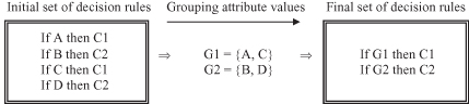
The other possibility of reducing the complexity of decision rules and decision trees is a process of grouping attribute values for categorical data. A large number of values cause a large space of data. There is a concern that useful patterns may not be detectable because of the insufficiency of training data, or that patterns will be detected but the model will be extremely complex.. To reduce the number of attribute values it is necessary to define appropriate groups. The number of possible splitting is large: for n values, there exist 2
n−1
− 1 nontrivial binary partitions. Even if the values are ordered, there are n − 1 “cut values” for binary splitting. A simple example, which shows the advantages of grouping categorical values in decision-rules reduction, is given in Figure
6.11
.
Figure 6.11.
Grouping attribute values can reduce decision-rules set.
C4.5 increases the number of grouping combinations because it does not include only binary categorical data, but also n-ary partitions. The process is iterative, starting with an initial distribution where every value represents a separate group, and then, for each new iteration, analyzing the possibility of merging the two previous groups into one. Merging is accepted if the information gain ratio (explained earlier) is nondecreasing. A final result may be two or more groups that will simplify the classification model based on decision trees and decision rules.
C4.5 was superseded in 1997 by a commercial system C5.0. The changes include
1.
a variant of boosting technique, which constructs an ensemble of classifiers that are then voted to give a final classification, and
2.
new data types such as dates, work with “not applicable” values, concept of variable misclassification costs, and mechanisms to pre-filter attributes.
C5.0 greatly improves scalability of both decision trees and rule sets, and enables successful applications with large real-world data sets. In practice, these data can be translated into more complicated decision trees that can include dozens of levels and hundreds of variables.
6.6 CART ALGORITHM & GINI INDEX
CART, as indicated earlier, is an acronym for Classification and Regression Trees. The basic methodology of divide and conquer described in C4.5 is also used in CART. The main differences are in the tree structure, the splitting criteria, the pruning method, and the way missing values are handled.
CART constructs trees that have only binary splits. This restriction simplifies the splitting criterion because there need not be a penalty for multi-way splits. Furthermore, if the label is binary, the binary split restriction allows CART to optimally partition categorical attributes (minimizing any concave splitting criteria) to two subsets of values in the number of attribute values. The restriction has its disadvantages, however, because the tree may be less interpretable with multiple splits occurring on the same attribute at the adjacent levels.