Authors: Mehmed Kantardzic
Data Mining (115 page)
The second operator that can be applied in every iteration of a GA is mutation. For our example, the mutation operator has a probability of 0.1%, which means that in the 1000 transformed bits, a mutation will be performed only once. Because we transformed only 20 bits (one population of 4 × 5 bits is transformed into another), the probability that a mutation will occur is very small. Therefore, we can assume that the strings CR
1
′ to CR
4
′ will stay unchanged with respect to a mutation operation in this first iteration. It is expected that only one bit will be changed for every 50 iterations.
That was the final processing step in the first iteration of the GA. The results, in the form of the new population CR
1
′ to CR
4
′, are used in the next iteration, which starts again with an evaluation process.
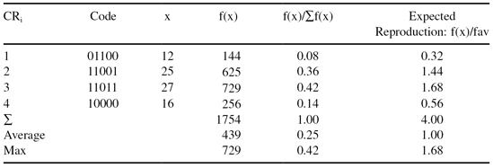
13.3.6 Evaluation (Second Iteration)
The process of evaluation is repeated in the new population. These results are given in Table
13.3
.
TABLE 13.3.
Evaluation of the Second Generation of Chromosomes
The process of optimization with additional iterations of the GA can be continued in accordance with Figure
13.3
. We will stop here with a presentation of computational steps for our example, and give some additional analyses of results useful for a deeper understanding of a GA.
Although the search techniques used in the GA are based on many random parameters, they are capable of achieving a better solution by exploiting the best alternatives in each population. A comparison of sums, and average and max values from Tables
13.2
and
13.3
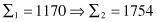
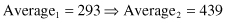
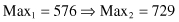
shows that the new, second population is approaching closer to the maximum of the function f(x). The best result obtained from the evaluation of chromosomes in the first two iterations is the chromosome CR3′ = 11011 and it corresponds to the feature’s value x = 27 (theoretically it is known that the maximum of f(x) is for x = 31, where f(x) reaches the value 961). This increase will not be obtained in each GA iteration, but on average, the final population is much closer to a solution after a large number of iterations. The number of iterations is one possible stopping criterion for the GA algorithm. The other possibilities for stopping the GA are when the difference between the sums in two successive iterations is less than the given threshold, when a suitable fitness value is achieved, and when the computation time is limited.
13.4 SCHEMATA
The theoretical foundations of GAs rely on a binary-string representation of solutions, and on the notation of a
schema
—a template allowing exploration of similarities among chromosomes. To introduce the concept of a schema, we have to first formalize some related terms. The search space Ω is the complete set of possible chromosomes or strings. In a fixed-length string
l,
where each bit (gene) can take on a value in the alphabet A of size
k,
the resulting size of the search space is
k
l
. For example, in binary-coded strings where the length of the string is 8, the size of the search space is 2
8
= 256. A string in the population S is denoted by a vector x ∈ Ω. So, in the previously described example, x would be an element of {0, 1}
8
. A schema is a similarity template that defines a subset of strings with fixed values in certain positions.
A schema is built by introducing a
don’t care
symbol (*) into the alphabet of genes. Each position in the scheme can take on the values of the alphabet (fixed positions) or a “don’t care” symbol. In the binary case, for example, the schemata of the length l are defined as H ∈ {0, 1, *}
l
. A schema represents all the strings that match it on all positions other than “*”. In other words, a schema defines a subset of the search space, or a hyperplane partition of this search space. For example, let us consider the strings and schemata of the length ten. The schema
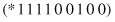
matches two strings

and the schema
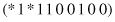
matches four strings

Of course, the schema
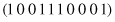
represents one string only, and the schema
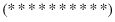
represents all strings of length 10. In general, the total number of possible schemata is (
k
+ 1)
l
, where
k
is the number of symbols in the alphabet and
l
is the length of the string. In the binary example of coding strings, with a length of 10, it is (2+1)
10
= 3
10
= 59049 different strings. It is clear that every binary schema matches exactly 2
r
strings, where r is the number of
don’t care
symbols in a schema template. On the other hand, each string of length m is matched by 2
m
different schemata.