Authors: Mehmed Kantardzic
Data Mining (26 page)
A general property necessary for any inductive principle including ERM is asymptotic
consistency
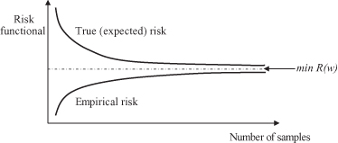
, which is a requirement that the estimated model converge to the true model or the best possible estimation, as the number of training samples grows large. An important objective of the SLT is to formulate the conditions under which the ERM principle is consistent. The notion of consistency is illustrated in Figure
4.4
. When the number of samples increases, empirical risk also increases while true, expected risk decreases. Both risks approach the common minimum value of the risk functional: min R(w) over the set of approximating functions, and for an extra large number of samples. If we take the classification problem as an example of inductive learning, the empirical risk corresponds to the probability of misclassification for the training data, and the expected risk is the probability of misclassification averaged over a large amount of data not included into a training set, and with unknown distribution.
Figure 4.4.
Asymptotic consistency of the ERM.
Even though it can be intuitively expected that for n → ∞ the empirical risk converges to the true risk, this by itself does not imply the consistency property, which states that minimizing one risk for a given data set will also minimize the other risk. To ensure that the consistency of the ERM method is always valid and does not depend on the properties of the approximating functions, it is necessary that consistency requirement should hold for all approximating functions. This requirement is known as nontrivial consistency. From a practical point of view, conditions for consistency are at the same time prerequisites for a good generalization obtained with the realized model. Therefore, it is desirable to formulate conditions for convergence of risk functions in terms of the general properties of a set of the approximating functions.
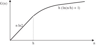
Let us define the concept of a
growth function
G(n) as a function that is either linear or bounded by a logarithmic function of the number of samples n. Typical behavior of the growth function G(n) is given in Figure
4.5
. Every approximating function that is in the form of the growth function G(n) will have a consistency property and potential for a good generalization under inductive learning, because empirical and true risk functions converge. The most important characteristic of the growth function G(n) is the concept of
VC dimension
. At a point n = h where the growth starts to slow down, it is a characteristic of a set of functions. If h is finite, then the G(n) function does not grow linearly for enough large training data sets, and it is bounded by a logarithmic function. If G(n) is only linear, then h → ∞, and no valid generalization through selected approximating functions is possible. The finiteness of h provides necessary and sufficient conditions for the quick convergence of risk functions, consistency of ERM, and potentially good generalization in the inductive-learning process. These requirements place analytic constraints on the ability of the learned model to generalize, expressed through the empirical risk. All theoretical results in the SLT use the VC dimension defined on the set of loss functions. But, it has also been proven that the VC dimension for theoretical loss functions is equal to the VC dimension for approximating functions in typical, inductive-learning tasks such as classification or regression.
Figure 4.5.
Behavior of the growth function G(n).
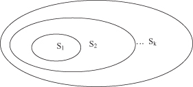
The ERM inductive principle is intended for relatively large data sets, namely, when the ratio n/h is large and the empirical risk converges close to the true risk. However, if n/h is small, namely, when the ratio n/h is less than 20, then a modification of the ERM principle is necessary. The inductive principle called SRM provides a formal mechanism for choosing a model with optimal complexity in finite and small data sets. According to SRM, solving a learning problem with a finite data set requires a priori specification of a structure on a set of approximating functions. For example, a set of functions S
1
is a subset of S
2
, and S
2
is a subset of S
3
. The set of approximating functions S
1
has the lowest complexity, but the complexity increases with each new superset S
2
, S
3
, … , S
k
. A simplified graphical representation of the structure is given in Figure
4.6
.
Figure 4.6.
Structure of a set of approximating functions.
For a given data set, the optimal model estimation is performed following two steps:
1.
selecting an element of a structure having optimal complexity, and
2.
estimating the model based on the set of approximating functions defined in a selected element of the structure.
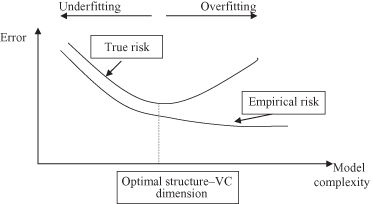
Through these two steps the SRM provides a quantitative characterization of the trade-off between the complexity of approximating functions and the quality of fitting the training data. As the complexity increases (increase of the index k for S
k
), the minimum empirical risk decreases, and the quality of fitting the data improves. But estimated true risk, measured through the additional testing data set, has a convex form, and in one moment it moves in a direction opposite that of the empirical risk, as shown in Figure
4.7
. The SRM chooses an optimal element of the structure that yields the minimal guaranteed bound on the true risk.
Figure 4.7.
Empirical and true risk as a function of h (model complexity).
In practice, to implement the SRM approach, it is necessary to be able to
1.
calculate or estimate the VC dimension for any element S
k
of the structure, and then
2.
minimize the empirical risk for each element of the structure.
For most practical inductive-learning methods that use nonlinear approximating functions, finding the VC dimension analytically is difficult, as is the nonlinear optimization of empirical risk. Therefore, rigorous application of the SRM principle cannot only be difficult but, in many cases, impossible with nonlinear approximations. This does not, however, imply that the SLT is impractical. There are various heuristic procedures that are often used to implement SRM implicitly. Examples of such heuristics include early stopping rules and weight initialization, which are often used in artificial neural networks. These heuristics will be explained together with different learning methods in the following chapters. The choice of an SRM-optimization strategy suitable for a given learning problem depends on the type of approximating functions supported by the learning machine. There are three commonly used optimization approaches:
1.
Stochastic Approximation (or Gradient Descent).
Given an initial estimate of the values for the approximating functions of parameter w, the optimal parameter values are found by repeatedly updating them. In each step, while computing the gradient of the risk function, the updated values of the parameters cause a small movement in the direction of the steepest descent along the risk (error) function.
2.
Iterative Methods.
Parameter values w are estimated iteratively so that at each iteration the value of the empirical risk is decreased. In contrast to stochastic approximation, iterative methods do not use gradient estimates; instead, they rely on a particular form of approximating functions with a special iterative parameter.
3.
Greedy Optimization.
The greedy method is used when the set of approximating functions is a linear combination of some basic functions. Initially, only the first term of the approximating functions is used and the corresponding parameters optimized. Optimization corresponds to minimizing the differences between the training data set and the estimated model. This term is then held fixed, and the next term is optimized. The optimization process is repeated until values are found for all parameters w and for all terms in the approximating functions.
These typical optimization approaches and also other more specific techniques have one or more of the following problems:
1.
Sensitivity to Initial Conditions.
The final solution is very sensitive to the initial values of the approximation function parameters.
2.
Sensitivity to Stopping Rules.
Nonlinear approximating functions often have regions that are very flat, where some optimization algorithms can become “stuck” for a long time (for a large number of iterations). With poorly designed stopping rules these regions can be interpreted falsely as local minima by the optimization algorithm.
3.
Sensitivity to Multiple Local Minima.
Nonlinear functions may have many local minima, and optimization methods can find, at best, one of them without trying to reach global minimum. Various heuristics can be used to explore the solution space and move from a local solution toward a globally optimal solution.
Working with finite data sets, SLT reaches several conclusions that are important guidelines in a practical implementation of data-mining techniques. Let us briefly explain two of these useful principles. First, when solving a problem of inductive learning based on finite information, one should keep in mind the following general commonsense principle: Do not attempt to solve a specified problem by indirectly solving a harder general problem as an intermediate step. We are interested in solving a specific task, and we should solve it directly. Following SLT results, we stress that for estimation with finite samples, it is always better to solve a specific learning problem rather than attempt a general one. Conceptually, this means that posing the problem directly will then require fewer samples for a specified level of accuracy in the solution. This point, while obvious, has not been clearly stated in most of the classical textbooks on data analysis.
Second, there is a general belief that for inductive-learning methods with finite data sets, the best performance is provided by a model of optimal complexity, where the optimization is based on the general philosophical principle known as Occam’s razor. According to this principle, limiting the model complexity is more important than using true assumptions with all details. We should seek simpler models over complex ones and optimize the trade-off between model complexity and the accuracy of the model’s description and fit to the training data set. Models that are too complex and fit the training data very well or too simple and fit the data poorly are both not good models because they often do not predict future data very well. Model complexity is usually controlled in accordance with Occam’s razor principle by a priori knowledge.