Data Mining (23 page)
Authors: Mehmed Kantardzic
while the χ
2
test is

TABLE 3.8.
Contingency Table for Intervals [0, 7.5] and [7.5, 10]

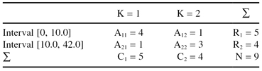
Selected intervals should be merged into one because, for the degree of freedom d = 1, χ
2
= 0.834 < 2.706 (for α = 0.1). In our example, with the given threshold value for χ
2
, the algorithm will define a final discretization with three intervals: [0, 10], [10, 42], and [42, 60], where 60 is supposed to be the maximum value for the feature F. We can assign to these intervals coded values 1, 2, and 3 or descriptive linguistic values low, medium, and high.
Additional merging is not possible because the χ
2
test will show significant differences between intervals. For example, if we attempt to merge the intervals [0, 10] and [10, 42]—contingency table is given in Table
3.9
—and the test results are E
11
= 2.78, E
12
= 2.22, E
21
= 2.22, E
22
= 1.78, and χ
2
= 2.72 > 2.706, the conclusion is that significant differences between two intervals exist, and merging is not recommended.
TABLE 3.9.
Contingency Table for Intervals [0, 10] and [10, 42]
3.8 CASE REDUCTION
Data mining can be characterized as a secondary data analysis in the sense that data miners are not involved directly in the data-collection process. That fact may sometimes explain the poor quality of raw data. Seeking the unexpected or the unforeseen, the data-mining process is not concerned with optimal ways to collect data and to select the initial set of samples; they are already given, usually in large numbers, with a high or low quality, and with or without prior knowledge of the problem at hand.
The largest and the most critical dimension in the initial data set is the number of cases or samples or, in other words, the number of rows in the tabular representation of data. Case reduction is the most complex task in data reduction. Already, in the preprocessing phase, we have elements of case reduction through the elimination of outliers and, sometimes, samples with missing values. But the main reduction process is still ahead. If the number of samples in the prepared data set can be managed by the selected data-mining techniques, then there is no technical or theoretical reason for case reduction. In real-world data-mining applications, however, with millions of samples available, that is not the case.
Let us specify two ways in which the sampling process arises in data analysis. First, sometimes the data set itself is merely a sample from a larger, unknown population, and sampling is a part of the data-collection process. Data mining is not interested in this type of sampling. Second (another characteristic of data mining), the initial data set represents an extremely large population and the analysis of the data is based only on a subset of samples. After the subset of data is obtained, it is used to provide some information about the entire data set. It is often called estimator and its quality depends on the elements in the selected subset. A sampling process always causes a sampling error. Sampling error is inherent and unavoidable for every approach and every strategy. This error, in general, will decrease when the size of subset increases, and it will theoretically become nonexistent in the case of a complete data set. Compared with data mining of an entire data set, practical sampling possesses one or more of the following advantages: reduced cost, greater speed, greater scope, and sometimes even higher accuracy. As yet there is no known method of sampling that ensures that the estimates of the subset will be equal to the characteristics of the entire data set. Relying on sampling nearly always involves the risk of reaching incorrect conclusions. Sampling theory and the correct selection of a sampling technique can assist in reducing that risk, but not in eliminating it.
There are various strategies for drawing a representative subset of samples from a data set. The size of a suitable subset is determined by taking into account the cost of computation, memory requirements, accuracy of the estimator, and other characteristics of the algorithm and data. Generally, a subset size can be determined so that the estimates for the entire data set do not differ by more than a stated margin error in more than δ of the samples. By setting up a probability inequality P(|e − e
0
| ≥ ε) ≤ δ, we solve it for the subset of sample size n, and for a given value ε (confidence limit) and δ (where 1 − δ is the confidence level). The parameter e stands for an estimate from the subset and it is generally a function of the subset size n, while e
0
stands for the true value obtained from entire data set. However, e
0
is usually unknown too. In this case, a practical way to determine the required size of the data subset can be done as follows: In the first step we select a small preliminary subset of samples of size m. Observations made based on this subset of data will be used to estimate e
0
. After replacing e
0
in the inequality, it is solved for n. If n ≥ m, additional n − m samples are selected in the final subset for analysis. If n ≤ m no more samples are selected, and the preliminary subset of data is used as the final.
One possible classification of sampling methods in data mining is based on the scope of application of these methods, and the main classes are
1.
general-purpose sampling methods
2.
sampling methods for specific domains.
In this text we will introduce only some of the techniques that belong to the first class because they do not require specific knowledge about the application domain and may be used for a variety of data-mining applications.
Systematic sampling
is the simplest sampling technique. For example, if we want to select 50% of a data set, we could take every other sample in a database. This approach is adequate for many applications and it is a part of many data-mining tools. However, it can also lead to unpredicted problems when there are some regularities in the database. Therefore, the data miner has to be very careful in applying this sampling technique.
Random sampling
is a method by which every sample from an initial data set has the same chance of being selected in the subset. The method has two variants:
random sampling without replacement
and
random sampling with replacement
. Random sampling without replacement is a popular technique in which n distinct samples are selected from N initial samples in the data set without repetition (a sample may not occur twice). The advantages of the approach are simplicity of the algorithm and nonexistence of any bias in a selection. In random sampling with replacement, the samples are selected from a data set such that all samples are given an equal chance of being selected, no matter how often they already have been drawn, that is, any of the samples may be selected more than once. Random sampling is not a one-time activity in a data-mining process. It is an iterative process, resulting in several randomly selected subsets of samples. The two basic forms of a random sampling process are as follows.
1.
Incremental Sampling.
Mining incrementally larger random subsets of samples that have many real-world applications helps spot trends in error and complexity. Experience has shown that the performance of the solution may level off rapidly after some percentage of the available samples has been examined. A principal approach to case reduction is to perform a data-mining process on increasingly larger random subsets, to observe the trends in performances, and to stop when no progress is made. The subsets should take big increments in data sets, so that the expectation of improving performance with more data is reasonable. A typical pattern of incremental subsets might be 10, 20, 33, 50, 67, and 100%. These percentages are reasonable, but can be adjusted based on knowledge of the application and the number of samples in the data set. The smallest subset should be substantial, typically, no fewer than 1000 samples.
2.
Average Sampling.
When the solutions found from many random subsets of samples of cases are
averaged
or
voted
, the combined solution can do as well or even better than the single solution found on the full collection of data. The price of this approach is the repetitive process of data mining on smaller sets of samples and, additionally, a heuristic definition of criteria to compare the several solutions of different subsets of data. Typically, the process of voting between solutions is applied for classification problems (if three solutions are class1 and one solution is class2, then the final voted solution is class1) and averaging for regression problems (if one solution is 6, the second is 6.5, and the third 6.7, then the final averaged solution is 6.4). When the new sample is to be presented and analyzed by this methodology, an answer should be given by each solution, and a final result will be obtained by comparing and integrating these solutions with the proposed heuristics.
Two additional techniques,
stratified sampling
and
inverse sampling
, may be convenient for some data-mining applications. Stratified sampling is a technique in which the entire data set is split into nonoverlapping subsets or strata, and sampling is performed for each different stratum independently of another. The combination of all the small subsets from different strata forms the final, total subset of data samples for analysis. This technique is used when the strata are relatively homogeneous and the variance of the overall estimate is smaller than that arising from a simple random sample. Inverse sampling is used when a feature in a data set occurs with rare frequency, and even a large subset of samples may not give enough information to estimate a feature value. In that case, sampling is dynamic; it starts with the small subset and it continues until some conditions about the required number of feature values are satisfied.
For some specialized types of problems, alternative techniques can be helpful in reducing the number of cases. For example, for time-dependent data the number of samples is determined by the frequency of sampling. The sampling period is specified based on knowledge of the application. If the sampling period is too short, most samples are repetitive and few changes occur from case to case. For some applications, increasing the sampling period causes no harm and can even be beneficial in obtaining a good data-mining solution. Therefore, for time-series data the windows for sampling and measuring features should be optimized, and that requires additional preparation and experimentation with available data.
3.9 REVIEW QUESTIONS AND PROBLEMS
1.
Explain what we gain and what we lose with dimensionality reduction in large data sets in the preprocessing phase of data mining.
2.
Use one typical application of data mining in a retail industry to explain monotonicity and interruptability of data-reduction algorithms.
3.
Given the data set X with three input features and one output feature representing the classification of samples, X: