Understanding Sabermetrics (28 page)
Read Understanding Sabermetrics Online
Authors: Gabriel B. Costa,Michael R. Huber,John T. Saccoma
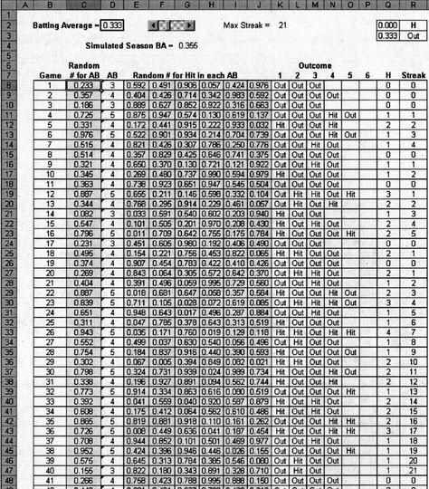
Figure 12.1 A simulation of a hitting streak
Based on observed data, we input the batting average. We can then run a simulation and determine a hitting streak and simulated batting average. With technology today, thousands of seasonal simulations can be run in minutes. Suppose we input Joe DiMaggio’s batting average. During his famous streak, Joe had a batting average of .408 and a slugging average of .717. If we input this batting average into our simulation, it is likely that we still would not see a hitting streak anywhere close to 56 games.
How good of a model is our simulation? First, it does not update the batting average after each game, although this could be incorporated with some effort. Varying the batting average from game to game would give insight into whether or not the batter gets into a slump. Our simulation uses actual data from DiMaggio’s 1941 season (specifically, the number of at-bats per game). This appears to be reasonable for a general approximation. The biggest point that one might bring up concerns the pitcher. During the 1941 streak, DiMaggio faced four future Hall of Fame pitchers, and yet he was successful. It is difficult to predict whether a given pitcher will be “in the zone” during a particular game. Some great batters claim they never have success against certain pitchers. However, conducting a simulation offers some insight into situations where a sabermetrical analysis might not.
RegressionAs a second example of analyzing the game of baseball beyond sabermetrics, let’s consider salary data. Baseball agents, general managers, and arbitrators use statistics in determining how lucrative a contract to a player should receive. Oftentimes they employ regression in determining a baseline salary. We will develop a regression model to predict future earnings based on past performances. As a basic example, consider two variables,
x
, and
y
, that represent two quantities, say batting average and salary, respectively. If the salary is based solely on batting average, we could use a linear relationship, such as y =
β
0
+
β
1
x. The slope
β
1
and
y
-intercept
β
0
determine a straight line. In this example, the batting average (
x
) is the independent variable, and the salary (
y
), is the dependent variable. Given a set of values for
x
, we could predict values for
y
in a linear fashion. In the context of our example, if we know the player’s batting average, we multiply it by a constant
β
1
, add another constant
β
0
, and determine the salary. This is known as a simple linear regression model.
x
, and
y
, that represent two quantities, say batting average and salary, respectively. If the salary is based solely on batting average, we could use a linear relationship, such as y =
β
0
+
β
1
x. The slope
β
1
and
y
-intercept
β
0
determine a straight line. In this example, the batting average (
x
) is the independent variable, and the salary (
y
), is the dependent variable. Given a set of values for
x
, we could predict values for
y
in a linear fashion. In the context of our example, if we know the player’s batting average, we multiply it by a constant
β
1
, add another constant
β
0
, and determine the salary. This is known as a simple linear regression model.
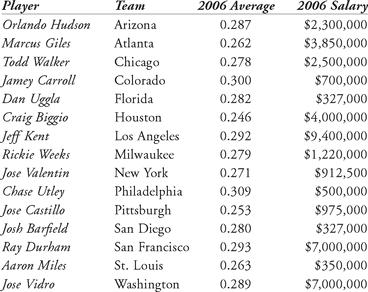
Table 12.3 Batting average and salary data for 2006 National League second basemen
Often players are compared to other players of equal ability to determine salary. Consider the 2006 National League second basemen. In Table 12.3, we list fifteen of the sixteen second basemen who played the most games for their respective teams in 2006, followed by their batting averages, and their 2006 salaries. Brandon Phillips was the regular second baseman for the Cincinnati Reds, batting .276. Based solely on the batting averages of his peers, what should Phillips’ salary be?
The first step in developing a regression analysis that involves just two variables is to try to develop a trend for the data. We therefore create a scatter plot of the observed data (see Figure 12.2), with the independent variable, batting average, on the
x
-axis, and the dependent variable, salary, on the
y
-axis.
x
-axis, and the dependent variable, salary, on the
y
-axis.
An initial look at the chart seems to reveal no pattern. Is there a trend? Using the method of least squares, we develop a trend line (the best fit of the data to a line). The principle behind the least squares method tells us that the vertical deviation of a point from a line is equal to the
y
-value of the point minus the
y
-value of the line for a given
x
-value. In other words, it is equal to
y-
(
β
0
+β
1
x
) This difference is calculated for all (
x
,
y
) pairs of the data, and then each vertical deviation is squared and summed. The scatter plot is shown again in Figure 13.3, with the trend line. The equation for this line is given by
y
= 24,481,096
x
- 4,071,161. The point estimates of
β
1
and
β
0
are called the least squares estimates and are those values which minimize the sum of the squared difference between
y
and (
β
0
+β
1
x)
y
-value of the point minus the
y
-value of the line for a given
x
-value. In other words, it is equal to
y-
(
β
0
+β
1
x
) This difference is calculated for all (
x
,
y
) pairs of the data, and then each vertical deviation is squared and summed. The scatter plot is shown again in Figure 13.3, with the trend line. The equation for this line is given by
y
= 24,481,096
x
- 4,071,161. The point estimates of
β
1
and
β
0
are called the least squares estimates and are those values which minimize the sum of the squared difference between
y
and (
β
0
+β
1
x)
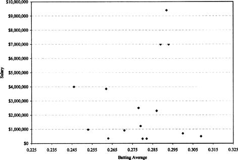
Figure 12.2 Scatterplot of batting average / salary data
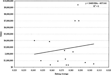
Figure 12.3 Scatterplot with trend line
How good is this trend line? In truth, for this model it’s not very good at all. The equation basically states that a ballplayer would have to owe over four million dollars if he never had an at-bat, or if his batting average remained at .000. Substituting Brandon Phillips’ batting average of .276, he should have made $2,685,621. However, both Rickie Weeks and Todd Walker had batting averages close to but greater than Phillips’, but their 2006 salaries were less than the prediction for Phillips. Further, only five players have salaries above the predicted line.
What happened? First, trying to predict something as complicated as a salary based on only one independent variable is probably not going to work. Second, the fifteen data points were spread out, with a maximum value of $9,400,000 and a minimum value of $327,000 (the league minimum). The mean for the data is $2,757,433, but the standard deviation is $2,915,708, which is larger than the mean! The player with the highest batting average had one of the lowest salaries, and several high-paid players had lower batting averages. Additionally, there were only 15 sets of data points. To get a more accurate prediction we need more data.
Let’s not give up yet. We wish to find a parameter that has a lower variability in the regression model. If the variability is small, the data points will tend to be closer to the predicted regression line, and the sum of the squared error (vertical deviation) will be small. Most statistics texts give thorough explanations of the sum of squared error, often denoted by “SSE,” and the reader should consult a statistics text for greater details. Our purpose here is to say that a useful estimate of the variance of the data can be calculated from the SSE:
 where σ
 2
2
is the estimate of the variance, SSE is the sum of squared error, and
n
is the number of data points. The denominator in the above expression gives the number of degrees of freedom associated with the variance estimate. The SSE can often be thought of as how the variation in the dependent variable
y
is unexplained in the linear relationship. Or, how much the data cannot be modeled by a linear relationship. If the SSE or variance estimate σ
2
is relatively high, as in the above example, the data probably cannot be modeled with a linear regression model. We can quantitatively measure the total amount of variation in the observed
y
-values by calculating the “SST,” the total sum of squares, where SST equals the sum of the
y
-values squared minus the sum of the
y
-values squared divided by
n
:
 for each -value. After calculating the SSE and SST, we can determine the coefficient of determination, or
r
2
value, as follows:

2is the estimate of the variance, SSE is the sum of squared error, and
n
is the number of data points. The denominator in the above expression gives the number of degrees of freedom associated with the variance estimate. The SSE can often be thought of as how the variation in the dependent variable
y
is unexplained in the linear relationship. Or, how much the data cannot be modeled by a linear relationship. If the SSE or variance estimate σ
2is relatively high, as in the above example, the data probably cannot be modeled with a linear regression model. We can quantitatively measure the total amount of variation in the observed
y
-values by calculating the “SST,” the total sum of squares, where SST equals the sum of the
y
-values squared minus the sum of the
y
-values squared divided by
n
:
r
2
value, as follows:
Other books
Jilted in January by Kate Pearce
Starstruck - Book Two by Gemma Brooks
The Prince of Midnight by Laura Kinsale
A Cowboy Unmatched by Karen Witemeyer
Dragon Ultimate by Christopher Rowley
Enchantment by Nikki Jefford
The Meadow by James Galvin
Blood of Angels by Marie Treanor
For Authentication Purposes by Amber L. Johnson
Be Mine by Jennifer Crusie