Data Mining (7 page)
Authors: Mehmed Kantardzic
1.9 REFERENCES FOR FURTHER STUDY
Berson, A., S. Smith, K. Thearling,
Building Data Mining Applications for CRM
, McGraw-Hill, New York, 2000.
The book is written primarily for the business community, explaining the competitive advantage of data-mining technology. It bridges the gap between understanding this vital technology and implementing it to meet a corporation’s specific needs. Basic phases in a data-mining process are explained through real-world examples.
Han, J., M. Kamber,
Data Mining: Concepts and Techniques
, 2nd edition, Morgan Kaufmann, San Francisco, CA, 2006.
This book gives a sound understanding of data-mining principles. The primary orientation of the book is for database practitioners and professionals, with emphasis on OLAP and data warehousing. In-depth analysis of association rules and clustering algorithms is an additional strength of the book. All algorithms are presented in easily understood pseudo-code, and they are suitable for use in real-world, large-scale data-mining projects, including advanced applications such as Web mining and text mining.
Hand, D., H. Mannila, P. Smith,
Principles of Data Mining
, MIT Press, Cambridge, MA, 2001.
The book consists of three sections. The first, foundations, provides a tutorial overview of the principles underlying data-mining algorithms and their applications. The second section, data-mining algorithms, shows how algorithms are constructed to solve specific problems in a principled manner. The third section shows how all of the preceding analyses fit together when applied to real-world data-mining problems.
Olson D., S. Yong,
Introduction to Business Data Mining
, McGraw-Hill, Englewood Cliffs, NJ, 2007.
Introduction to Business Data Mining
was developed to introduce students, as opposed to professional practitioners or engineering students, to the fundamental concepts of data mining. Most importantly, this text shows readers how to gather and analyze large sets of data to gain useful business understanding. The authors’ team has had extensive experience with the quantitative analysis of business as well as with data-mining analysis. They have both taught this material and used their own graduate students to prepare the text’s data-mining reports. Using real-world vignettes and their extensive knowledge of this new subject, David Olson and Yong Shi have created a text that demonstrates data-mining processes and techniques needed for business applications.
Westphal, C., T. Blaxton,
Data Mining Solutions: Methods and Tools for Solving Real-World Problems
, John Wiley, New York, 1998.
This introductory book gives a refreshing “out-of-the-box” approach to data mining that will help the reader to maximize time and problem-solving resources, and prepare for the next wave of data-mining visualization techniques. An extensive coverage of data-mining software tools is valuable to readers who are planning to set up their own data-mining environment.
2
PREPARING THE DATA
Chapter Objectives
- Analyze basic representations and characteristics of raw and large data sets.
- Apply different normalization techniques on numerical attributes.
- Recognize different techniques for data preparation, including attribute transformation.
- Compare different methods for elimination of missing values.
- Construct a method for uniform representation of time-dependent data.
- Compare different techniques for outlier detection.
- Implement some data preprocessing techniques.
2.1 REPRESENTATION OF RAW DATA
Data samples introduced as rows in Figure 1.4 are basic components in a data-mining process. Every sample is described with several features, and there are different types of values for every feature. We will start with the two most common types:
numeric
and
categorical
. Numeric values include real-value variables or integer variables such as age, speed, or length. A feature with numeric values has two important properties: Its values have an order relation (2 < 5 and 5 < 7) and a distance relation (d [2.3, 4.2] = 1.9).
In contrast, categorical (often called symbolic) variables have neither of these two relations. The two values of a categorical variable can be either equal or not equal: They only support an equality relation (Blue = Blue, or Red ≠ Black). Examples of variables of this type are eye color, sex, or country of citizenship. A categorical variable with two values can be converted, in principle, to a numeric binary variable with two values: 0 or 1. A categorical variable with
n
values can be converted into
n
binary numeric variables, namely, one binary variable for each categorical value. These coded categorical variables are known as “dummy variables” in statistics. For example, if the variable eye color has four values (black, blue, green, and brown), they can be coded with four binary digits.
| Feature Value | Code |
| Black | 1000 |
| Blue | 0100 |
| Green | 0010 |
| Brown | 0001 |
Another way of classifying a variable, based on its values, is to look at it as a continuous variable or a discrete variable.
Continuous variables are also known as
quantitative
or
metric variables
. They are measured using either an interval scale or a ratio scale. Both scales allow the underlying variable to be defined or measured theoretically with infinite precision. The difference between these two scales lies in how the 0 point is defined in the scale. The 0 point in the
interval scale
is placed arbitrarily, and thus it does not indicate the complete absence of whatever is being measured. The best example of the interval scale is the temperature scale, where 0 degrees Fahrenheit does not mean a total absence of temperature. Because of the arbitrary placement of the 0 point, the ratio relation does not hold true for variables measured using interval scales. For example, 80 degrees Fahrenheit does not imply twice as much heat as 40 degrees Fahrenheit. In contrast, a
ratio scale
has an absolute 0 point and, consequently, the ratio relation holds true for variables measured using this scale. Quantities such as height, length, and salary use this type of scale. Continuous variables are represented in large data sets with values that are numbers—real or integers.
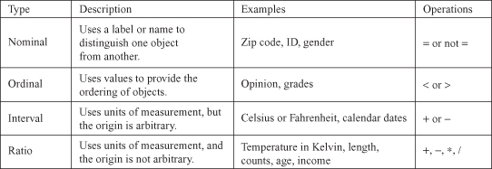
Discrete variables
are also called qualitative variables. Such variables are measured, or their values defined, using one of two kinds of nonmetric scales—
nominal
or
ordinal
. A nominal scale is an orderless scale, which uses different symbols, characters, and numbers to represent the different states (values) of the variable being measured. An example of a nominal variable, a utility, customer-type identifier with possible values is residential, commercial, and industrial. These values can be coded alphabetically as A, B, and C, or numerically as 1, 2, or 3, but they do not have metric characteristics as the other numeric data have. Another example of a nominal attribute is the zip code field available in many data sets. In both examples, the numbers used to designate different attribute values have no particular order and no necessary relation to one another.
An
ordinal scale
consists of ordered, discrete gradations, for example, rankings. An ordinal variable is a categorical variable for which an order relation is defined but not a distance relation. Some examples of an ordinal attribute are the rank of a student in a class and the gold, silver, and bronze medal positions in a sports competition. The ordered scale need not be necessarily linear; for example, the difference between the students ranked fourth and fifth need not be identical to the difference between the students ranked 15th and 16th. All that can be established from an ordered scale for ordinal attributes with greater-than, equal-to, or less-than relations. Typically, ordinal variables encode a numeric variable onto a small set of overlapping intervals corresponding to the values of an ordinal variable. These ordinal variables are closely related to the linguistic or fuzzy variables commonly used in spoken English, for example, AGE (with values young, middle aged, and old) and INCOME (with values low-middle class, upper middle class, and rich). More examples are given in Figure
2.1
, and the formalization and use of fuzzy values in a data-mining process are given in Chapter 14.
Figure 2.1.
Variable types with examples.
A special class of discrete variables is periodic variables. A
periodic variable
is a feature for which the distance relation exists, but there is no order relation. Examples are days of the week, days of the month, or days of the year. Monday and Tuesday, as the values of a feature, are closer than Monday and Thursday, but Monday can come before or after Friday.
Finally, one additional dimension of classification of data is based on its behavior with respect to time. Some data do not change with time, and we consider them
static data
. On the other hand, there are attribute values that change with time, and this type of data we call
dynamic
or
temporal data
. The majority of data-mining methods are more suitable for static data, and special consideration and some preprocessing are often required to mine dynamic data.
Most data-mining problems arise because there are large amounts of samples with different types of features. Additionally, these samples are very often high dimensional, which means they have extremely large number of measurable features. This additional dimension of large data sets causes the problem known in data-mining terminology as “the curse of dimensionality.” The “curse of dimensionality” is produced because of the geometry of high-dimensional spaces, and these kinds of data spaces are typical for data-mining problems. The properties of high-dimensional spaces often appear counterintuitive because our experience with the physical world is in a low-dimensional space, such as a space with two or three dimensions. Conceptually, objects in high-dimensional spaces have a larger surface area for a given volume than objects in low-dimensional spaces. For example, a high-dimensional hypercube, if it could be visualized, would look like a porcupine, as in Figure
2.2
. As the dimensionality grows larger, the edges grow longer relative to the size of the central part of the hypercube. Four important properties of high-dimensional data affect the interpretation of input data and data-mining results.
1.
The size of a data set yielding the same density of data points in an n-dimensional space increases exponentially with dimensions. For example, if a one-dimensional (1-D) sample containing n data points has a satisfactory level of density, then to achieve the same density of points in k dimensions, we need n
k
data points. If integers 1 to 100 are values of 1-D samples, where the domain of the dimension is [0, 100], then to obtain the same density of samples in a 5-D space we will need 100
5
= 10
10
different samples. This is true even for the largest real-world data sets; because of their large dimensionality, the density of samples is still relatively low and, very often, unsatisfactory for data-mining purposes.
Figure 2.2.
High-dimensional data look conceptually like a porcupine.

2.
A larger radius is needed to enclose a fraction of the data points in a high-dimensional space. For a given fraction of samples, it is possible to determine the edge length
e
of the hypercube using the formula where p is the prespecified fraction of samples, and d is the number of dimensions. For example, if one wishes to enclose 10% of the samples (p = 0.1), the corresponding edge for a 2-D space will be
e
2
(0.1) = 0.32, for a 3-D space
e
3
(0.1) = 0.46, and for a 10-D space
e
10
(0.1) = 0.80. Graphical interpretation of these edges is given in Figure
2.3
.
Figure 2.3.
Regions enclose 10% of the samples for one-, two-, and three-dimensional spaces.
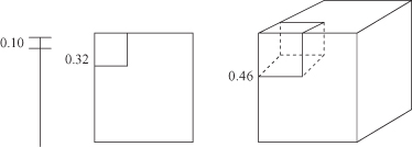
This shows that a very large neighborhood is required to capture even a small portion of the data in a high-dimensional space.
3.
Almost every point is closer to an edge than to another sample point in a high-dimensional space. For a sample of size n, the expected distance D between data points in a d-dimensional space is
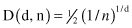
For example, for a 2-D space with 10,000 points the expected distance is D(2,10,000) = 0.005 and for a 10-D space with the same number of sample points D(10,10,000) = 0.4. Keep in mind that the maximum distance from any point to the edge occurs at the center of the distribution, and it is 0.5 for normalized values of all dimensions.
4.
Almost every point is an outlier. As the dimension of the input space increases, the distance between the prediction point and the center of the classified points increases. For example, when d = 10, the expected value of the prediction point is 3.1 standard deviations away from the center of the data belonging to one class. When d = 20, the distance is 4.4 standard deviations. From this standpoint, the prediction of every new point looks like an outlier of the initially classified data. This is illustrated conceptually in Figure
2.2
, where predicted points are mostly in the edges of the porcupine, far from the central part.