Data Mining (74 page)
Authors: Mehmed Kantardzic
Essentially, in determining the similarity between two values, any categorical measure is filling the entries of this matrix. For example, the overlap measure sets the diagonal entries to 1 and the off-diagonal entries to 0, that is, the similarity is 1 if the values match and 0 if the values mismatch. Additionally, measures may use the following information in computing a similarity value (all the measures in this paper use only this information):
1.
f(a), f(b), f(c), and f(d), the frequencies of the values in the data set;
2.
N, the size of the data set; and
3.
n, the number of values taken by the attribute (4 in the case above).
We will present, as an illustrative example, only one additional measure of similarity for categorical data,
Goodall3
, because it shows good performances on average for a variety of experiments with different data sets. That does not mean that some other measures such as Eskin, Lin, Smirnov, or Burnaby will not be more appropriate for a specific data set. The
Goodall3 measure
, given in Table
9.4
, assigns a high similarity if the matching values are infrequent regardless of the frequencies of the other values.
The range of
S
k
(
X
k
;
Y
k
) for matches in the
Goodall3
measure is , with
the minimum value being attained if
X
k
is the only value for attribute A
k
and maximum value is attained if
X
k
occurs only twice.
TABLE 9.4.
Goodall3 Similarity Measure for Categorical Attributes

There are some advanced distance measures applicable to categorical data, and also to numerical data, that take into account the effect of the surrounding or neighboring points in the n-dimensional spaces of samples. These surrounding points are called contexts. The similarity between two points, x
i
and x
j
, with the given context, is measured using the
mutual neighbor distance
(MND), which is defined as

where NN(x
i
, x
j
) is the neighbor number of x
j
with respect to x
i
. If x
i
is the closest point to x
j,
then NN(x
i
, x
j
) is equal to 1, if it is the second closest point, NN(x
i
, x
j
) is equal to 2, and so on. Figures
9.3
and
9.4
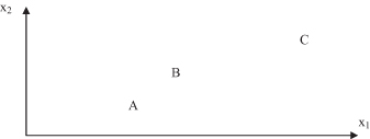
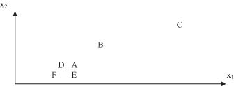
give an example of the computation and basic characteristics of the MND measure.
Figure 9.3.
A and B are more similar than B and C using the MND measure.

Figure 9.4.
After changes in the context, B and C are more similar than A and B using the MND measure.

Points in Figures
9.3
and
9.4
, denoted by A, B, C, D, E, and F, are 2-D samples with features x
1
and x
2
. In Figure
9.3
, the nearest neighbor of A is B using Euclidian distance, and B’s nearest neighbor is A. So,

If we compute the distance between points B and C, the results will be

Figure
9.4
was obtained from Figure
9.3
by adding three new points D, E, and F (samples in the data set). Now, because the context has changed, the distances between the same points A, B, and C have also changed:


The MND between A and B has increased by introducing additional points close to A, even though A and B have not moved. B and C points become more similar than points A and B. The MND measure is not a metric because it does not satisfy the triangle inequality. Despite this, MND has been successfully applied in several real-world clustering tasks.
In general, based on a distance measure between samples, it is possible to define a distance measure between clusters (set of samples). These measures are an essential part in estimating the quality of a clustering process, and therefore they are part of clustering algorithms. The widely used measures for distance between clusters C
i
and C
j
are
1.
D
min
(C
i
, C
j
) = min |p
i
− p
j
|, where p
i
∈ C
i
and p
j
∈ C
j
;
2.
D
mean
(C
i
, C
j
) = |m
i
− m
j
|, where m
i
and m
j
are centriods of C
i
and C
j
;
3.
D
avg
(C
i
, C
j
) = 1/(n
i
n
j
) ∑ ∑ |p
i
− p
j
|, where p
i
∈ C
i
and p
j
∈ C
j
, and n
i
and n
j
are the numbers of samples in clusters C
i
and C
j
; and
4.
D
max
(C
i
, C
j
) = max |p
i
− p
j
|, where p
i
∈ C
i
and p
j
∈ C
j
.