Data Mining (75 page)
Authors: Mehmed Kantardzic
9.3 AGGLOMERATIVE HIERARCHICAL CLUSTERING
In hierarchical-cluster analysis, we do not specify the number of clusters as a part of the input. Namely, the input to a system is (X, s), where X is a set of samples, and s is a measure of similarity. An output from a system is a hierarchy of clusters. Most procedures for hierarchical clustering are not based on the concept of optimization, and the goal is to find some approximate, suboptimal solutions, using iterations for improvement of partitions until convergence. Algorithms of hierarchical cluster analysis are divided into the two categories, divisible algorithms and agglomerative algorithms. A
divisible algorithm
starts from the entire set of samples X and divides it into a partition of subsets, then divides each subset into smaller sets, and so on. Thus, a divisible algorithm generates a sequence of partitions that is ordered from a coarser one to a finer one. An
agglomerative algorithm
first regards each object as an initial cluster. The clusters are merged into a coarser partition, and the merging process proceeds until the trivial partition is obtained: All objects are in one large cluster. This process of clustering is a bottom-up process, where partitions are from a finer one to a coarser one. In general, agglomerative algorithms are more frequently used in real-world applications than divisible methods, and therefore we will explain the agglomerative approach in greater detail.
Most agglomerative hierarchical clustering algorithms are variants of the
single-link
or
complete-link
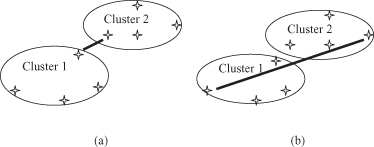
algorithms. These two basic algorithms differ only in the way they characterize the similarity between a pair of clusters. In the single-link method, the distance between two clusters is the
minimum
of the distances between all pairs of samples drawn from the two clusters (one element from the first cluster, the other from the second). In the complete-link algorithm, the distance between two clusters is the
maximum
of all distances between all pairs drawn from the two clusters. A graphical illustration of these two distance measures is given in Figure
9.5
.
Figure 9.5.
Distances for a single-link and a complete-link clustering algorithm. (a) Single-link distance; (b) complete-link distance.

In either case, two clusters are merged to form a larger cluster based on minimum-distance criteria. Although the single-link algorithm is computationally simpler, from a practical viewpoint it has been observed that the complete-link algorithm produces more useful hierarchies in most applications.
As explained earlier, the only difference between the single-link and complete-link approaches is in the distance computation. For both, the basic steps of the agglomerative clustering algorithm are the same. These steps are as follows:
1.
Place each sample in its own cluster. Construct the list of intercluster distances for all distinct unordered pairs of samples, and sort this list in ascending order.
2.
Step through the sorted list of distances, forming for each distinct threshold value d
k
a graph of the samples where pairs of samples closer than d
k
are connected into a new cluster by a graph edge. If all the samples are members of a connected graph, stop. Otherwise, repeat this step.
3.
The output of the algorithm is a nested hierarchy of graphs, which can be cut at the desired dissimilarity level forming a partition (clusters) identified by simple connected components in the corresponding subgraph.
Let us consider five points {x
1
, x
2
, x
3
, x
4
, x
5
} with the following coordinates as a 2-D sample for clustering:

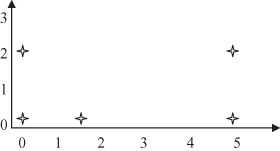
For this example, we selected 2-D points because it is easier to graphically represent these points and to trace all the steps in the clustering algorithm. The points are represented graphically in Figure
9.6
.
Figure 9.6.
Five two-dimensional samples for clustering.

The distances between these points using the Euclidian measure are


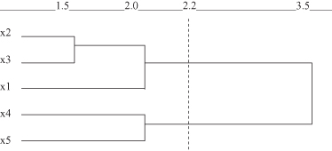
The distances between points as clusters in the first iteration are the same for both single-link and complete-link clustering. Further computation for these two algorithms is different. Using agglomerative single-link clustering, the following steps are performed to create a cluster and to represent the cluster structure as a dendrogram.
First x
2
and x
3
samples are merged and a cluster {x
2
, x
3
} is generated with a minimum distance equal to 1.5. Second, x
4
and x
5
are merged into a new cluster {x
4
, x
5
} with a higher merging level of 2.0. At the same time, the minimum single-link distance between clusters {x
2
, x
3
} and {x
1
} is also 2.0. So, these two clusters merge at the same level of similarity as x
4
and x
5
. Finally, the two clusters {x
1
, x
2
, x
3
} and {x
4
, x
5
} are merged at the highest level with a minimum single-link distance of 3.5. The resulting dendrogram is shown in Figure
9.7
.
Figure 9.7.
Dendrogram by single-link method for the data set in Figure
9.6
.

The cluster hierarchy created by using an agglomerative complete-link clustering algorithm is different compared with the single-link solution. First, x
2
and x
3
are merged and a cluster {x
2
, x
3
} is generated with the minimum distance equal to 1.5. Also, in the second step, x
4
and x
5
are merged into a new cluster {x
4
, x
5
} with a higher merging level of 2.0. Minimal single-link distance is between clusters {x
2
, x
3
}, and {x
1
} is now 2.5, so these two clusters merge after the previous two steps. Finally, the two clusters {x
1
, x
2
, x
3
} and {x
4
, x
5
} are merged at the highest level with a minimal complete-link distance of 5.4. The resulting dendrogram is shown in Figure
9.8
.